I like a lot the ANOVA-based answer by Stephan Kolassa. However, I would also like to offer a slightly different perspective.
First of all, consider the reason why you're testing for nonlinearity. If you want to test the assumptions of ordinary least squares to estimate the simple linear regression model, note that if you then want to use the estimated model to perform other tests (e.g., test whether the correlation between $X$ and $Y$ is statistically significant), the resulting test will be a composite test, whose Type I and Type II error rates won't be the nominal ones. This is one of multiple reasons why, instead than formally testing the assumptions of linear regression, you may want to use plots in order to understand if those assumptions are reasonable. Another reason is that the more tests you perform, the more likely you are to get a significant test result even if the null is true (after all, linearity of the relationship between $X$ and $Y$ is not the only assumption of the simple linear regression model), and closely related to this reason there's the fact that assumption tests have themselves assumptions!
For example, following Stephan Kolassa's example, let's build a simple regression model:
set.seed(1)
xx <- runif(100)
yy <- xx^2+rnorm(100,0,0.1)
plot(xx,yy)
linear.model <- lm(yy ~ xx)
The plot function for linear models shows a host of plots whose goal is exactly to give you an idea about the validity of the assumptions behind the linear model and the OLS estimation method. The purpose of the first of these plots, the residuals vs fitted plot, is exactly to show if there are deviations from the assumption of a linear relationship between the predictor $X$ and the response $Y$:
plot(linear.model)
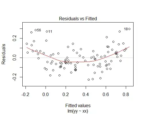
You can clearly see that there is a quadratic trend between fitted values and residuals, thus the assumption that $Y$ is a linear function of $X$ is questionable.
If, however, you are determined on using a statistical test to verify the assumption of linearity, then you're faced with the issue that, as noted by Stephan Kolassa, there are infinitely many possible forms of nonlinearity, so you cannot possibly devise a single test for all of them. You need to decide your alternatives and then you can test for them.
Now, if all your alternatives are polynomials, then you don't even need ANOVA, because by default R computes orthogonal polynomials. Let's test 4 alternatives, i.e., a linear polynomial, a quadratic one, a cubic one and a quartic one. Of course, looking at the residual vs fitted plot, there's not evidence for an higher than degree 2 model here. However, we include the higher degree models to show how to operate in a more general case. We just need one fit to compare all four models:
quartic.model <- lm(yy ~ poly(xx,4))
summary(quartic.model)
Call:
lm(formula = yy ~ poly(xx, 4))

Residuals:
      Min        1Q    Median        3Q       Max
-0.175678 -0.061429 -0.007403  0.056324  0.264612

Coefficients:
             Estimate Std. Error t value Pr(>|t|)
(Intercept)   0.33729    0.00947  35.617  < 2e-16 ***
poly(xx, 4)1  2.78089    0.09470  29.365  < 2e-16 ***
poly(xx, 4)2  0.64132    0.09470   6.772 1.05e-09 ***
poly(xx, 4)3  0.04490    0.09470   0.474    0.636
poly(xx, 4)4  0.11722    0.09470   1.238    0.219
As you can see, the p-values for the first and second degree term are extremely low, meaning that a linear fit is insufficient, but the p-values for the third and fourth term are much larger, meaning that third or higher degree models are not justified. Thus, we select the second degree model. Note that this is only valid because R is fitting orthogonal polynomials (don't try to do this when fitting raw polynomials!). The result would have been the same if we had used ANOVA. As a matter of fact, the squares of the t-statistics here are equal to the F-statistics of the ANOVA test:
linear.model <- lm(yy ~ poly(xx,1))
quadratic.model <- lm(yy ~ poly(xx,2))
cubic.model <- lm(yy ~ poly(xx,3))
anova(linear.model, quadratic.model, cubic.model, quartic.model)
Analysis of Variance Table

Model 1: yy ~ poly(xx, 1)
Model 2: yy ~ poly(xx, 2)
Model 3: yy ~ poly(xx, 3)
Model 4: yy ~ poly(xx, 4)
  Res.Df     RSS Df Sum of Sq       F    Pr(>F)
1     98 1.27901
2     97 0.86772  1   0.41129 45.8622 1.049e-09 ***
3     96 0.86570  1   0.00202  0.2248    0.6365
4     95 0.85196  1   0.01374  1.5322    0.2188
For example, 6.772^2 = 45.85998, which is not exactly 45.8622 but pretty close, taking into account numerical errors.
The advantage of the ANOVA test comes into play when you want to explore non-polynomial models, as long as they're all nested. Two or more models $M_1,\dots,M_N$ are nested if the predictors of $M_i$ are a subset of the predictors of $M_{i+1}$, for each $i$. For example, let's consider a cubic spline model with 1 interior knot placed at the median of xx. The cubic spline basis includes linear, second and third degree polynomials, thus the linear.model, the quadratic.model and the cubic.model are all nested models of the following spline.model:
spline.model <- lm(yy ~ bs(xx,knots = quantile(xx,prob=0.5)))
The quartic.model is not a nested model of the spline.model (nor is the vice versa true), so we must leave it out of our ANOVA test:
anova(linear.model, quadratic.model,cubic.model,spline.model)
Analysis of Variance Table

Model 1: yy ~ poly(xx, 1)
Model 2: yy ~ poly(xx, 2)
Model 3: yy ~ poly(xx, 3)
Model 4: yy ~ bs(xx, knots = quantile(xx, prob = 0.5))
  Res.Df     RSS Df Sum of Sq       F    Pr(>F)
1     98 1.27901
2     97 0.86772  1   0.41129 46.1651 9.455e-10 ***
3     96 0.86570  1   0.00202  0.2263    0.6354
4     95 0.84637  1   0.01933  2.1699    0.1440
Again, we see that a quadratic fit is justified, but we have no reason to reject the hypothesis of a quadratic model, in favour of a cubic or a spline fit alternative.
Finally, if you would like to test also non-nested model (for example, you would like to test a linear model, a spline model and a nonlinear model such as a Gaussian Process), then I don't think there are hypothesis tests for that. In this case your best bet is cross-validation.

