The sigmoid function in the logistic regression model precludes utilizing the close algebraic parameter estimation as in ordinary least squares (OLS). Instead nonlinear analytical methods, such as gradient descent or Newton's method will be used to minimize the cost function of the form:
$\text{cost}(\sigma(\Theta^\top {\bf x}),{\bf y})=\color{blue}{-{\bf y}\log(\sigma(\Theta^\top {\bf x}))}\color{red}{-(1-{\bf y})\log(1-\sigma(\Theta^\top {\bf x}))}$, where
$\large \sigma(z)=\frac{1}{1+e^{-\Theta^\top{\bf x}}}$, i.e. the sigmoid function. Notice that if $y=1$, we want the predicted probability, $\sigma(\Theta^\top x)$, to be high, and the minus sign in the blue part of the cost function will minimize the cost; contrarily, if $y=0$, only the red part of the equation comes into place, and the smaller $\sigma(\Theta^\top x)$, the closer the cost will be to zero.
Equivalently, we can maximize the likelihood function as:
$p({\bf y \vert x,\theta}) = \left(\sigma(\Theta^\top {\bf x})\right)^{\bf y}\,\left(1 - \sigma(\Theta^\top {\bf x})\right)^{1 -\bf y}$.
The sentence you quote, though, makes reference, I believe, to the relatively linear part of the sigmoid function:
Because the model can be expressed as a generalized linear model (see
below), for $0<p<1$, ordinary least squares can suffice, with R-squared
as the measure of goodness of fit in the fitting space. When $p=0$ or $1$,
more complex methods are required.
The logistic regression model is:
$$\text{odds(Y=1)} = \frac{p\,(Y=1)}{1\,-\,p\,(Y=1)} = e^{\,\theta_0 + \theta_1 x_1 + \cdots + \theta_p x_p} $$
or,
$\log \left(\text{odds(Y=1)}\right) = \log\left(\frac{p\,(Y=1)}{1\,-\,p\,(Y=1)}\right) = \theta_0 + \theta_1 x_1 + \cdots + \theta_p x_p=\Theta^\top{\bf X}\tag{*}$
Hence, this is "close enough" to an OLS model ($\bf y=\Theta^\top \bf X+\epsilon$) to be fit as such, and for the parameters to be estimated in closed form, provided the probability of $\bf y = 1$ (remember the Bernoulli modeling of the response variable in logistic regression) is not close to $0$ or $1$. In other words, while $\log\left(\frac{p\,(Y=1)}{1\,-\,p\,(Y=1)}\right)$ in Eq. * stays away from the asymptotic regions.
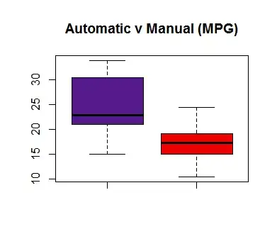
See for instance this interesting entry in Statistical Horizons, which I wanted to test with the mtcars dataset in R. The variable for automatic transmission am is binary, so we can regress it over miles-per-gallon mpg. Can we predict that a car model has automatic transmission based on its gas consumption?
If I go ahead, and just plow through the problem with OLS estimates I get a prediction accuracy of $75\%$ just based on this single predictor. And guess what? I get the exact same confusion matrix and accuracy rate if I fit a logistic regression.
The thing is that the output of OLS is not binary, but rather continuous, and trying to estimate the real binary $\bf y$ values, they are typically between $0$ and $1$, much like probability values, although not strictly bounded like in logistic regression (sigmoid function).
Here is the code:
> d = mtcars
> summary(as.factor(d$am))
 0  1
19 13
> fit_LR = glm(as.factor(am) ~ mpg, family = binomial, d)
> pr_LR = predict(fit, type="response")
>
> # all.equal(pr_LR, 1 / (1 + exp( - predict(fit_LR) ) ) ) - predict() is log odds P(Y =1)
>
> d$predict_LR = ifelse(pr_LR > 0.5, 1, 0)
> t_LR = table(d$am,d$predict_LR)
> (accuracy = (t_LR[1,1] + t_LR[2,2]) / sum(t))
[1] 0.75
>
> fit_OLS = lm(am ~ mpg, d)
> pr_OLS = predict(fitOLS)
> d$predict_OLS = ifelse(pr_OLS > 0.5, 1, 0)
> (t_OLS = table(d$am, d$predict_OLS))

     0  1
  0 17  2
  1  6  7
> (accuracy = (t[1,1] + t[2,2]) / sum(t_OLS))
[1] 0.75
The frequency of automatic v manual cars is pretty balanced, and the OLS model is good enough as a perceptron: