One way to deduce the simulated $n\log(n)$ behavior is through truncation.
Generally, for any distribution $F$ and $0\le \alpha\lt 1$ let $F_\alpha$ be truncated symmetrically in both tails so that for $F^{-1}(\alpha/2)\le x \le F^{-1}(1-\alpha/2),$
$$F_\alpha(x) = \min{\left(1, \frac{F(x) - \alpha/2}{1-\alpha}\right)}.$$
Let $E_\alpha$ be the expectation of $F_\alpha$ defined by
$$E_\alpha = \int_{\mathbb R} x\,\mathrm{d}F_\alpha(x).$$
Because the support of $F_\alpha$ is bounded, it has finite expectation and variance. The Central Limit Theorem tells us that for sufficiently large sample sizes $n,$ the sum of $n$ iid random variables with $F_\alpha$ for their common distribution is approximately Normal with mean $n E_\alpha.$ This approximate Normality implies the median of the sum distribution also is approximately $n E_\alpha.$
Now, the median of a sum of independent variables with distribution $F$ won't be quite the same as this approximate median: it must lie somewhere between the $1/2-\alpha/2$ and $1/2+\alpha/2$ quantiles. In the present case, where $F$ is nonzero in a neighborhood of its median, this means that by taking $\alpha$ sufficiently small (but still nonzero), we can make the median of $F_\alpha$ as close as we like to the median of $F=F_0.$
It remains only to find the mean of $F_\alpha$ in the question, where $F$ is the half-Cauchy distribution determined by
$$F(x) = \frac{2}{\pi}\int_0^x \frac{\mathrm{d}t}{1+t^2} = \frac{2}{\pi}\tan^{-1}(x)$$
for $x\ge 0.$
The ensuing calculations are straightforward. First,
$$E_\alpha = \frac{1}{1-\alpha}\int_{x_0}^{x_1} \frac{x\,\mathrm{d}x}{1+x^2} = \frac{1}{\pi(1-\alpha)} \log\frac{1+x_1^2}{1+x_0^2}$$
where $F(x_0) = \alpha/2$ and $F(x_1) = 1-\alpha/2.$ Thus
$$x_0 = \tan\left(\frac{\pi\alpha}{4}\right) \approx \frac{\pi\alpha}{4},\quad x_1 = \tan\left(\frac{\pi}{2}-\frac{\pi\alpha}{4}\right) = \frac{1}{x_0} \approx \frac{4}{\pi\alpha},$$
whence
$$E_\alpha \approx \frac{1}{\pi} \log \frac{1 + \left(\frac{4}{\pi\alpha}\right)^2}{1 + \left(\frac{\pi\alpha}{4}\right)^2} \approx \frac{2}{\pi}\log\left(\frac{4}{\pi\alpha}\right).$$
Finally, when taking a sample of size $n$ from $F$ we would like to ensure that most of the time the sample really is a sample of $F_\alpha,$ uncontaminated by any values in its tails. This happens with probability $(1-\alpha)^n.$ To make this chance exceed some threshold $1-\epsilon,$ with a tiny value of $\epsilon,$ we must have
$$\alpha \approx \frac{\epsilon}{n}.$$
Using this value in the foregoing gives
$$E_\alpha \approx \frac{2}{\pi}\log\left(\frac{4}{\pi\epsilon/n}\right) = \frac{2}{\pi}\left(\log\left(\frac{4}{\pi\epsilon}\right) + \log(n)\right).$$
Consequently, the median of the sum of $n$ iid half-Cauchy variables must be close to
$$nE_\alpha \approx \frac{2}{\pi}n\log(n) + \left(\frac{2}{\pi}\log\frac{4}{\pi\epsilon}\right)n.$$
For any desired $\epsilon\gt 0,$ we may choose $n$ so large that the value is dominated by the first term: that is how the $n\log n$ behavior arises. Moreover, now we have the implicit constant $2/\pi$ along with the asymptotic order of the error term, $O(n).$
Let the "relative median" be $nE_\alpha$ divided by $\left(2/\pi\right) n\log(n).$ Here is a plot of such relative medians as observed in 5,000 simulations of samples up to size 5,000. The reference red curve is a multiple of $1/\log(n),$ which this analysis indicates is proportional to the asymptotic relative error. The fit is good.
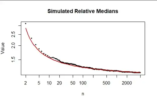
The R code to produce it can be used for additional simulation studies.
n.sim <- 5e3  # Simulation count
n <- 5e3      # Maximum sample size
X <- apply(apply(matrix(abs(rt(n*n.sim, 1)), n), 2, cumsum), 1, median)

N <- seq_len(n)[-1]        # Can't divide by n log(n) when n==0
X <- X[-1]
x.0 <- 2/pi * N * log(N)   # Theory
#
# Plot the relative medians.
#
plot(N, X / x.0, xlab="n", log="xy", cex=0.5, pch=19,
     ylab="Value",
     main="Simulated Relative Medians")
#
# Draw a reference curve.
#
fit <- lm(X / x.0 - 1 ~ 0 + I(1/log(N)))
summary(fit)
b <- coefficients(fit)[1]
curve(1 + b/log(n) , add=TRUE, xname="n", lwd=2, col="Red")
