For $n$ events, here is a $O(n\log(n))$ algorithm that uses simple, common tools.
For simplicity, let's normalize the times so that the start of sales is time $0$ and the end is time $1$. The normalized times themselves are $$0 \le t_1 \le t_2\le \cdots \le t_n \le 1.$$ Let $n(t)$ be the cumulative distribution through time $t$: $$n(t) = \#\{i\,|\, t_i \le t\}.$$ The number of events in the interval $(t-dt, t]$ of length $dt \ge 0$ therefore is $$\#(t-dt, dt]=n(t) - n(t-dt).$$ Such intervals are wholly included within the range of times $[0,1]$ when $dt \le t \le 1$. I will interpret the "proportion" of intervals with more than $k$ events as the proportion of this time: $$p(dt,k) = \frac{1}{1-dt}\int_{dt}^1 \mathcal{I}(n(t) - n(t-dt) \ge k) dt.$$ ($\mathcal{I}$ is the binary indicator function.)
For a given count $k \gt 0$ and proportion $1-\alpha$ (such as $\alpha=0.1$ for $90\%$ of the time), the question asks to find the smallest possible $dt$ for which $p(dt, k) \ge 1-\alpha.$ In particular, $dt$ is a zero of the (discontinuous but monotonic) function $$f(dt) = p(dt, k) - (1-\alpha).$$ A good root finder will efficiently discover such as $dt$. (If you wish, you may conduct a binary search instead.)
Here are illustrative plots for a synthetic dataset with $n=500,000$ in the course of one month, comparable to the situation posited in the question.
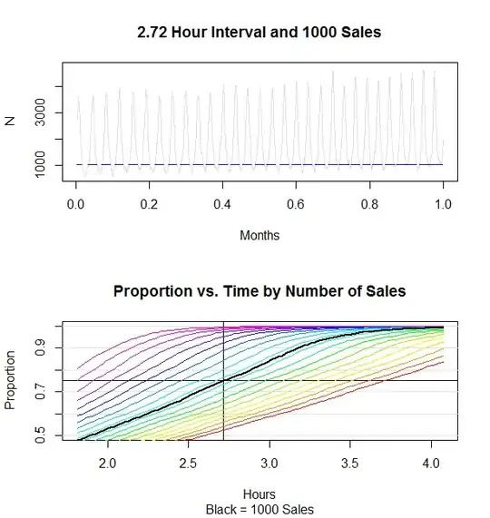
Code reproduced below found a solution for $k=1000$ purchases and $\alpha=0.25$; it is $2.72$ hours.
The top figure plots $n(t) - n(t-dt)$ for $dt = 2.72\text{ hours}$ = $2.72/(30\times 24)$ $\approx 0.00377\text{ months}.$ The blue horizontal line is located at a count (height) of $k=1000$. Only the segments at times where the preceding width-$dt$ interval contains $k$ or more purchases are shown. Collectively they comprise exactly $1-\alpha=75\%$ of the month (starting from time $dt$ and ending at time $1$). This graph perhaps is even more useful than the answer, because it reveals potentially important details, such as the trend over time.
The bottom graph illustrates this by plotting the total proportion of time against the time interval $dt$ for various values of $k$. The lower red and yellow curves plot values of $k$ largerthan $1000$ while the higher blue and purle curves plot values of $k$ smaller than $1000$. The black curve is the plot for $k=1000$. The value $1-\alpha=0.75$ appears as a black horizontal line. The interval where the black curve crosses this line is the solution, $2.72$ hours. It should now be visually evident how this problem amounts to finding a crossing (or zero) of a function.
It takes $O(n\log(n))$ time to sort the events, which is the core calculation in computing $n(t)$. A binary search or decent root finder will take $O(\log(n))$ iterations, each one taking $O(\log(n))$ time for an evaluation (in principle: the R implementation is a bit worse, but is simple to implement).
Here is the R code to produce the synthetic dataset (which oscillates daily and has a slight upward trend) and compute this solution. integrate implements the function $f$ (but divides its values by $n$). It simply samples the unit interval at a large number of equally spaced points. uniroot is the built-in root finder to find the interval. It took only $25$ iterations to find a solution precise to $10^{-8}$, requiring less than $0.1$ seconds to complete. Because these data are so numerous, the solution cannot be appreciably greater than the smallest possible value of $dt$ that works (as the previous plots confirm).
#
# Proportion of time in (dx, 1] that intervals of width `dx` contain at least `y` events.
#
integrate <- function(y, dx, fun, n.points=10001) {
  x <- seq(dx, 1, length.out=n.points)
  mean(f(x) - f(x-dx) >= y * (1-dx))
}
#
# Synthesize the data.
#
n <- 500000
set.seed(17)
dt <- rgamma(n+1, shape=1/10, rate=exp(0:n/n * 1/5)*(1.5 + sin(30*2*pi*0:n/n)))
#
# Normalize them.
#
times <- (cumsum(dt) / sum(dt))[1:n]
#
# Compute the cumulative distribution.
#
f <- ecdf(times)
#
# Specify `k` and `alpha`, then find `dt`.
#
k.0 <- 1000
alpha <- 0.25
fit <- uniroot(function(dx) integrate(k.0/n, dx, f) - (1-alpha), lower=0, upper=1, tol=1e-8)
