If you have performance measures per individual class (and individual models in your case), you could report those along/instead of reporting the prediction performance over all classes. For example, you could report the ROC curve, the AUC, EER, etc. for each class individually, and this does not necessarily depend on having underlying individual models. The first two mentioned metrics have the advantage of capturing the model power without employing a concrete threshold yet, and with the latter, the threshold is still automatically determined. Reporting the FRR and FAR per individual class (using a specifically chosen threshold) would be an option too.
In case you have too many classes in your data to report performance on class level you could instead report meta-statistics about those performances like mean, standard deviation, quantiles of AUC, EER, etc. An example would be boxplots showing AUC, EER, etc. for all classes - even a boxplot over FAR and FRR might make sense in some cases. While not giving details about which classes are predicted well or badly, this still captures the variation of performance across classes.
Most ML tools already provide the functionality for computation of such statistics alongside evaluation, so you don't necessarily need to do this on your own. Here's a small example using SVMs with 3 class classification and statistics on individual class basis in R with the caret package:
library(caret)
library(plyr)
library(pROC)

# example problem, 3 class classification
model <- train(x = iris[,1:4],
        iris[,5],
        method = 'svmLinear',
        metric = 'Kappa',
        trControl = trainControl(method = 'repeatedcv',
                                number = 10,
                                repeats = 20,
                                returnData = F,
                                returnResamp = 'final',
                                savePredictions = T,
                                classProbs = T),
        tuneGrid = expand.grid(C=3**(-3:3)))
plot(model, scales=list(x=list(log=3)))
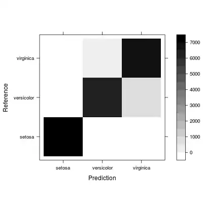
The overall confusion matrix already gives some insights to class confusion (you might want to use the relative representation instead):
# confusion accross partitions and repeats
conf <- confusionMatrix(data = model$pred$pred, reference=model$pred$obs)
print(conf)
levelplot(conf$table, col.regions=gray(100:0/100)) # absolute confusion over partitions and repeats
levelplot(sweep(conf$table, MARGIN = 2, STATS = colSums(conf$table), FUN = '/'), col.regions=gray(100:0/100)) # relative confusion over partitions and repeats
ROC curves can be calculated for individual classes (in this example only if the predictions been preserved during cross validation):
# compute ROC for each individual class
rocs <- llply(unique(model$pred$obs), function(cls) {
    roc(predictor = model$pred[[as.character(cls)]], response = model$pred$obs)
})

# report ROCs for individual classes in one figure
plot(rocs[[1]])
lines(rocs[[2]], col=2, lty=2)
lines(rocs[[3]], col=3, lty=3)
# ...
# compute some statistics per class
statistics <- ldply(rocs, function(cROC) {
    cAUC <- cROC$auc
    cEER <- cROC$sensitivities[which.min(abs(cROC$sensitivities-cROC$specificities))]
    # you could add further metrics here, like FAR, FRR for specific thresholds
    # ...
    data.frame(auc=cAUC, eer=cEER)
})
print(statistics)
Calculation numeric statistics could be done by class as well:
         .id       auc       eer
1     setosa 1.0000000 1.0000000
2 versicolor 0.9839534 0.9291429
3  virginica 0.9852129 0.9338571
...
Finally, meta-statistics of those metrics over all classes could be calculated and displayed (in case there are too many classes to be reported individually):
# compute some meta-statistics in case there are too many classes
print(summary(statistics))
boxplot(statistics[-1])
I hope this in fact addresses your questions. BTW: if you struggle getting good results with certain individual models due to having few positive but many negative samples in the associated training set you could consider adding sample/error weights during model training, or utilizing e.g. up/-downsampling.


