7

This Exercise is particularly important to me because so far I believe to have a rather poor understanding on how to compute the joint probability distribution.

Problem: Let $X$ be a RV with density $f(x)= \frac{1}{\pi\sqrt{x(1-x)}}$ for $x \in (0,1)$ and $Y$ be a RV with Exponential Distribution (standard, parameter 1). Assuming that $X,Y$ are independent I am supposed to find the joint distribution of $U=XY, \ V=(1-X)Y$


My approach: Although I couldn't rigorously proof it I think I can state that $(X,Y)$ has joint probability density given by $m(x,y)= \frac{1}{\pi \sqrt{x(1-x)}}e^{-y}$ for $(x,y) \in (0,1) \times (0, \infty)$

My idea was now to compute for an arbitrary bounded continuous $g:\mathbb{R^2} \to \mathbb{R}$ $$E(g(U,V)) = \int_{\mathbb{R^2}}g(u,v) h(u,v)dudv $$ and hope that I can find a density function $h$.

$$E(g(U,V))=E(g(XY,(1-X)Y)) \\ \overset{3)}= \int_{\mathbb{R}^2}g(xy,(1-x)y) \frac{1}{\pi \sqrt{x(1-x)}}e^{-y}1_{(x,y) \in (0,1) \times (0 , \infty)} dx dy \\ = \int_{(0,1) \times (0, \infty)} g(xy,(1-x)y) \frac{1}{\pi \sqrt{x(1-x)}}e^{-y} dx dy =:I$$

Choosing the obvious transformation/substitution $(u,v)=(xy,(1-x)y)$ I get $(u,v) \in (0, \infty) \times (0, \infty)$ and $x= \frac{u}{u+v},y=u+v$ for the Jacobi Matrix I obtain $$J= \begin{pmatrix} \frac{v}{(u+v)^2} & \frac{-u}{(u+v)^2} \\ 1 & 1 \end{pmatrix} \implies |\det J| = \frac{1}{u+v}>0 $$ So finally I would obtain for the above integral denoted as $I$ that $$I= \int_{(0, \infty)^2} g(u,v) \underbrace{\frac{1}{\pi(\sqrt{\frac{u}{u+v}(1-\frac{u}{u+v})}}e^{-(u+v)} \frac{1}{u+v}}dudv \\ = \int_{(0, \infty)^2} g(u.v) \frac{1}{\pi \sqrt{uv}} e^{-(u+v)}dudv$$


Questions: 1) The obvious question of course if the above is correct or not

2) Do I need to do anything more? Or just state that the distribution of $(U,V)$ is given by the strange underbraced term on the last integral?

3) Given the density function of $(X,Y)$ (assuming my formula in the first paragraph is correct) why is this equation true? Intuitively I don't see why this should hold given the more standard formula $$E(f(X))= \int_{\mathbb{R}^d} f(x) P_X(dx)$$

Additional Question (optional): I am very new to this topic and have little to no to experience, please if you know of a more elegant way to approach the solution I would gladly know about it.
whuber
  • 281,159
  • 54
  • 637
  • 1,101
Spaced
  • 383
  • 2
  • 12
  • Update: I think my integration limits are wrong because I said $v=(1-x)y$ where $x \in (0,1)$ and $y \in (0, \infty)$ it follows that $v \in (0, \infty)$ which is good, because that makes the Determinant of the Integral much better defined (no division by zero possible). I will update that. – Spaced Apr 23 '16 at 15:16
  • 1
    (1) Because both $u$ and $v$ are positive, you can substantially simplify the "strange underbraced term". (2) In question 3, what do you mean by "this equation"? (3) The [calculus of differential forms](http://stats.stackexchange.com/a/101298/919) is arguably "more elegant." It's certainly simpler! – whuber Apr 23 '16 at 16:49
  • Thanks a lot @whuber, I have done further simplifications. For my question 3 I highlighted it in the above question, meaning the 3) above the = sign. I wondered because I do understand that $$E(f((X,Y)))= \int f(x,y)h(x,y)dxdy $$ where $h$ is a density function of $(X,Y)$. However I do not understand why I can still use the same density function if I "change" $X,Y$ slightly for example I used something in the nature $$E(f(X+Y,XY))=\int f(x+y,xy)h(x,y)dxdy $$ i.e. I did not change the density function at all. Since you didn't comment on it, I suppose my calculations are indeed correct? – Spaced Apr 23 '16 at 17:13
  • Conclusion: $(U,V)$ has density given by $1_{(u,v) \in (0, \infty )^2} \frac{1}{\pi \sqrt{ uv}}e^{-(u+v)}$, additionally the random variables $U,V$ are independent because if I denote $$h(u,v)=1_{(u,v) \in (0, \infty )^2} \frac{1}{\pi \sqrt{ uv}}e^{-(u+v)} $$ then $h(u,v)=h_1(u)h_2(v)$ where $$ h_1(u)=1_{u \in (0, \infty)} \frac{1}{\sqrt{\pi u}} e^{-u}, \ h_2(v)= 1_{v \in (0, \infty)} \frac{1}{\sqrt{ \pi v }}e^{-v} $$ and $h_1, h_2$ are densities on $U$ respectively $V$. – Spaced Apr 23 '16 at 17:30

1 Answers1

2

Statistical reasoning provides an elegant solution.

Because the integral of $f$ is used to define inverse trig functions, one is immediately tempted to interpret $X=\sin^2(A)$ for a random variable $A$ ranging from (say) $0$ to $\pi/2$. Substituting $\sin(a)$ for $x$ in $f$ gives

$$f(x)\,\mathrm{d}x = f(\sin^2(a))\mathrm{d}\left(\sin^2(a)\right) = \frac{2\sin(a)\cos(a)\,\mathrm{d}a}{\pi\sqrt{\sin^2(a)(1-\sin^2(a))}}=\frac{2}{\pi}\mathrm{d}a.$$

This reveals $X$ as the squared sine of a uniformly distributed angle on $[0,\pi/2)$. Consequently $1-X=\cos^2(A)$ is its squared cosine.

Recall (this is familiar from the study of the Normal distribution and related distributions of statistical importance) that an Exponential variable $Y$ has the same distribution as half the sum of squares of two independent standard Normal variables $Z_1$ and $Z_2$. In the plane, the ordered pair $\mathbf{Z}=(Z_1,Z_2)$ has a standard bivariate Normal distribution, showing that $Y$ is half the squared length of $\mathbf{Z}$, $$Y=1/2\,|\mathbf{Z}|^2.$$

Consequently

$$U=XY = 1/2\,\sin^2(A)|\mathbf{Z}|^2 = 1/2\,\left(\sin(a)|\mathbf{Z}|\right)^2$$

and

$$V=(1-X)Y = 1/2\,\cos^2(A)|\mathbf{Z}|^2 = 1/2\,\left(\cos(a)|\mathbf{Z}|\right)^2.$$

Those expressions that have been squared are the very components of $\mathbf{Z}$ itself:

$$U = 1/2\,Z_1^2,\ V=1/2\,Z_2^2.$$

Apparently $U$ and $V$ are independent and their distributions are both--by definition--half a $\chi^2(1)$ distribution. It is now easy to write down their joint distribution any way you wish: as a PDF, CDF, characteristic function, moment-generating function, cumulant-generating function, etc. But it's probably most revealing to have expressed them in this familiar statistical form.


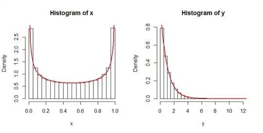
A quick simulation supports these conclusions: by simulating $U$ and $V$ independently as proportional to $\chi^2(1)$ variates and solving

$$Y=U+V;\ X=U/Y$$

we can see whether $X$ and $Y$ have the distributions originally assumed of them. A quick check--which could be formally verified with a goodness of fit test (like a chi-squared test)--is to overplot the histograms of the simulated $X$ and $Y$ with the density functions. They should match, up to a small amount of random variation in the areas of the histogram bars. They do.

Figure

Here is the R code that made this figure.

n <- 1e5
set.seed(17)

u <- 1/2 * rchisq(n, df=1)
v <- 1/2 * rchisq(n, df=1)
y <- u + v
x <- u / y

par(mfrow=c(1,2))
hist(x, freq=FALSE)
curve(1 / (pi * sqrt(x*(1-x))), col="Red", lwd=2, add=TRUE)
hist(y, freq=FALSE)
curve(exp(-x), col="Red", lwd=2, add=TRUE)
whuber
  • 281,159
  • 54
  • 637
  • 1,101