1

I am conducting a least square regression using the python library numpy. When I run OLS (ordinary least square regression) over just the variable IE6 I get this output (with the key takeaway being that the coefficient is negative):

=============================================================================
variable     coefficient     std. Error      t-statistic     prob.
==============================================================================
const          -0.632626      0.184070     -3.436882      0.001209
IE6            -11.845141      8.695507     -1.362214      0.179360
==============================================================================
Models stats                         Residual stats
==============================================================================
R-squared             0.036488         Durbin-Watson stat   1.635514
Adjusted R-squared    0.016825         Omnibus stat         12.433490
F-statistic           1.855627         Prob(Omnibus stat)   0.001996
Prob (F-statistic)    0.179360          JB stat              43.784881
Log likelihood       -47.743508         Prob(JB)             0.000000
AIC criterion         1.950726         Skew                 0.052388
BIC criterion         2.026484         Kurtosis             7.538025
==============================================================================

Yet when I add two additional variables percent and percent_m, the sign of the coefficient switches to positive. Apparently, I don't understand the mechanics of OLS well enough, because this switch perplexes me.

Here is the output of the second regression:

==============================================================================
variable     coefficient     std. Error      t-statistic     prob.
==============================================================================
const          -1.511714      0.417273     -3.622840      0.000725
percent           1.852263      0.710854      2.605689      0.012313
percent_m          -2.657285      1.233789     -2.153760      0.036533
IE6             9.625211      6.499429      1.480932      0.145442
==============================================================================
Models stats                         Residual stats
==============================================================================
R-squared             0.282134         Durbin-Watson stat   1.896240
Adjusted R-squared    0.219711         Omnibus stat         8.682105
F-statistic           4.519698         Prob(Omnibus stat)   0.013023
Prob (F-statistic)    0.003660          JB stat              14.649562
Log likelihood       -40.238818         Prob(JB)             0.000659
AIC criterion         1.774071         Skew                 0.366255
BIC criterion         1.963466         Kurtosis             5.521377
==============================================================================
chl
  • 50,972
  • 18
  • 205
  • 364
Spencer
  • 221
  • 3
  • 11
  • 2
    Did you take a look at this related question: [Regression coefficients that flip sign after including other predictors](http://stats.stackexchange.com/q/1580/930)? – chl Jan 02 '12 at 22:38

3 Answers3

6

Notice that IE6 is not significantly different from 0 in either analysis. Most of what you are seeing is random variation around 0. Some correlation between IE6 and the other 2 variables can easily influence the direction of the random variation.

Greg Snow
  • 46,563
  • 2
  • 90
  • 159
  • +1 for being more observant. However, even when there are real relationships between the predictors and the response, multicollinearity can cause the sign to flip, as I know you know well. – gung - Reinstate Monica Jan 03 '12 at 00:07
  • 1
    @gung yes multicollinearity can cause the sign of a significant coefficient to change, but the degree of multicollinearity needed to make the change is much smaller when the coefficient size is small compared to its standard deviation. – Greg Snow Jan 03 '12 at 00:47
4

Update: I agree with Greg Snow that neither predictor in the question is significant, and that it is easier for the sign to bounce back and forth when it isn't actually related. Nonetheless, I think this is an important and potentially confusing issue that is worth explaining clearly. So I've fleshed out my answer in the hopes of making this dynamic more comprehensible.

What can be going on in situations like this, is that your predictor variables are correlated with each other, a condition called 'multicollinearity'. Consider a case with just two predictors (x1 and x2) that are both positively correlated with the response variable when assessed individually (albeit one more so than the other), but are also both highly correlated with each other. When x1 is entered into the model, it does it's best to predict y, but, being imperfect, there is some residual variance left over. Then x2 is entered. This is not the same as x2 trying to predict y on its own, but rather predicting y given that x1 is already in the model, and the output is telling you about the nature of that relationship. More technically, the estimated slope values $(\hat\beta_1, \hat\beta_2)$ are those values that taken together minimize the sum of squared errors ($\Sigma (y_i-\hat{y}_i)^2$). It is quite possible that the relationship between x2 and y is negative when x1 is in the model (i.e., $\hat\beta_2<0$), but that when x2 is correlated with y on its own, it shows up as a positive relationship. This is because its strong correlation with x1 and x1's strong correlation with y outweighs the negative relationship between x2 and y.

This is demonstrated in the following:

set.seed(321) 
N = 100
     # generate standard normal random data
x1 = rnorm(N);     x2 = rnorm(N)

     # this makes the predictors correlated
conversion_matrix = rbind(c(1.0, 0.8),
                           c(0.8, 1.0))
X = cbind(x1, x2) %*% conversion_matrix
     # assign correlated data to original variables
x1 = X[,1];     x2 = X[,2]

     # this is the 'true' model
y = .9*x1 - .8*x2 + rnorm(N, mean=0, sd=.10)

Note that my two predictors are strongly correlated, and both are strongly related to y, but one slightly more so than the other, and x2 is (in truth) negatively related to y. However, that latter statement is not apparent from looking at only the marginal relationships, as can be seen in this scatterplot matrix:

enter image description here

Although the slope values are somewhat shallow, the relationships are strong, positive, and highly 'significant'. However, look at the relationship between x2 and y when we control for x1:

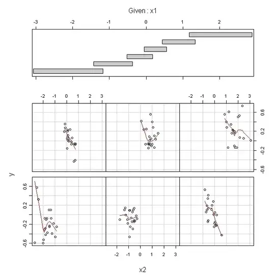
enter image description here

Although coplots are always a bit messy to read, it is clear that the relationship between x2 and y is negative once we've controlled for x1. (How to read this coplot: the data are grouped into partially overlapping 'slices' by their x1 values; there should be approximately the same number in each slice, and the ranges are displayed in the top panel. The bottom panels plot y against x2 within each of the slices.)

model12 = lm(y~x1+x2)
coef(model12)
(Intercept)          x1          x2 
0.01645146   0.88632611 -0.79373947

In addition, note that the slopes for both x1 and x2 have changed, relative to the values displayed on the scatterplot matrix above. Moreover, these values are much closer to the true values from the data generating process that we started with.

gung - Reinstate Monica
  • 132,789
  • 81
  • 357
  • 650
  • Greg and gung have done a nice job of trying to explain a complicated phenomenon succintly. To go deeper into the topic, you could read up on *suppressor variables* and *partial correlation*. – rolando2 Jan 03 '12 at 19:09
1

Another way to view this issue is with vectors.

Think of the entire list of output values,y, as a single point you're trying to represent, in a high dimensional space (1 dimension per sample). Then think of each list of input values, x1 and x2 as basis vector in this same space.

The least squares regression adds together linear combinations of the basis vectors to try to get "as close as possible" to the target point, and closeness here is measured in the usual way, sum of squares.

The problem is that the basis vectors are not orthogonal.

With orthogonal bases, adding a new coordinate doesn't affect the others. the best x1 coordinate is independent of the best x2 coordinate.

On a skewed grid, where your basis vectors are not orthogonal, adding a basis vector affects the best fit coordinates of the other bases (it changes the fit coefficients)

Imagine we have two samples (so the high dimensional space I mentioned before is 2D) and:

y=(2,3)
x1=(1,0)

So the coefficient for x1 (the distance to go in the x1 direction) is:

c1 = 2

Now if we add a second input value:

x2=(1,1)

Then recalculate the coefficients (the distance to go in each of the x directions)?

c1 = -1
c2 = 3

c1 has flipped signs, just like in your data. to keep that from happening start by normalize your inputs unit length:

x1 = (1,0)
x2 = (0.707,0.707)

Then remove any component of the new vector that lines up with any of the old (already in use) vectors:

x2' = x2-dot(x1,x2)*x1
x2' = unit(x2)

=> x2' = (0,1)

Now you can fit x2' without knowing, or changing c1:

c1 = 2
c2' = 3

So it solves your sign change problem. orthogonalize first, then the fit coefficients won't change at all.

This is the basis of fourier series and orthogonal polynomials

mdaoust
  • 141
  • 3