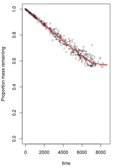
I have several datasets. Each dataset holds the masses of objects that have been subject to physical wear, expressed as a proportion of their original mass ($w$), and the amount of time that the object was exposed to physical wear ($t$). I assume that objects wear at a constant rate while they are exposed to wear, and that within a dataset, wear-rates are approximately Normally-distributed.
At some amount of wear, objects fail due to wear. Failed objects cannot be recovered, and so are not recorded in any dataset.
For each dataset, I wish to estimate:
- The mean wear-rate of objects within that dataset ($\mu$)
- The proportion of wear at which objects fail and become unobservable ($b$).
I have attempted a Bayesian approach to to estimating these parameters, as suggested in this question. When the dataset is affected by truncation, my current approach generates upward-biased estimates of $\mu$, and very imprecise estimates of $b$.
Code (R and JAGS):
points <- 1000

time <- runif(points, 0, 20000)  ## anything up to 20,000 days. For a
                                  # dataset unaffected by
                                  # truncation, drop this to ~ 5000.
wearRates <- rnorm(points, (0.022/365), (0.0022/365))
## typical wear-rates
wear <- 1-(time*wearRates)
losspoint <- 0.55  ## failure when 55% of initial mass remains
observable <- wear > losspoint

allPoints <- data.frame(time, wear, observable)
data <- subset(allPoints, observable == TRUE)

with(data, plot.default(wear ~ time
                  , ylim = c(0,1)
                  , ylab="Proportion mass remaining",
                  , col=rgb(0,0,0, alpha=0.2)
                  , pch = 16)
                  )
lines(lowess(data$time, data$wear, f = 0.1), type = "l", col=2, lwd = 2)
## plot of the generated data, with Lowess smoother. The smoother line
 # will show an 'elbow' if the dataset is strongly affected by truncation.

library(R2jags)
library(coda)

modelString="
model {
   #Likelihood
   for (i in 1:n) {
      w[i]~dlnorm(-mu*t[i], (sigma^2)*t[i]^2)T(b,1)
   }

# Priors
   mu ~ dnorm(0.022, 1.0E-8)
   b ~ dunif(0, 1)
   sigma ~ dunif(0,100)

# Derived parameters
   annualWear <- mu*365
}
"

writeLines(modelString, con="./wearModel.txt")

data.list <- with(data, list(w = wear, t = time, n = nrow(data)))
## dataset trimmed to a manageable size for JAGS
params <- c("mu", "b", "sigma", "annualWear")
nChains = 3
burnInSteps = 3000
thinSteps = 10
numSavedSteps = 15000
nIter = ceiling(burnInSteps+(numSavedSteps * thinSteps)/nChains)

data.r2jags <- jags(data = data.list,
                    inits = NULL,
                    parameters.to.save = params,
                    model.file = "./wearModel.txt",
                    n.chains = nChains,
                    n.iter = nIter,
                    n.burnin = burnInSteps,
                    n.thin = thinSteps)

print(data.r2jags)

plot(as.mcmc(data.r2jags))
Example:
Here is a dataset affected by data-truncation due to wear (generated using the code above). Truncation is obvious from the characteristic 'elbow' in the Lowess smoother line. The value of b will therefore be near the lowest value of $w$ in this dataset (the value of $b$ is set to 0.55 in this example).
However, the posterior densities for b do not peak near the lowest value of $w$ as I expected them to. Also, the values of annualWear (which is defined as $\mu$*365) are estimated to be higher than they should be - annualWear is set to 0.022, not around 0.0265. annualWear appears to be more-accurately estimated in datasets that are unaffected by truncnation.
What am I doing wrong here?

