General Linear Model without the main effects

Question

In the post here, a contributor (dmk38) makes an interesting, and may I add a very commonsense observation, that to include or not to include the main effects in an interaction model containing the product term should be guided by theory and hypothesis that is being tested.

I have a similar situation where the product term (X1*X2) is significant. However, when I use X1, X2 and X1*X2 in the model, the latter becomes insignificant. I am using the general linear model in SPSS.

I am only interested in the significance of X1*X2 interaction and I can justify it based on my hypothesis that I am assessing the relationship between X1 and Y and how this relationship is moderated by X2. I already know that there is a strong correlation between X1 and Y (so there is little point of assessing the main effect of X1 on Y in the model.)

I am certainly not 'fishing around' for significance but just tried the two approaches above i.e. one with the main effects and one without the main effects. Both models contained the product term.

Question: Given the confusion in the above post, I am unsure if the above approach which leaves out the main effects is a valid approach (though it makes intuitive sense to a non-statistician like me!)

Answer 1

If the values of X1 and X2 are positive and positively correlated with Y, then of course X1*X2 will be significant when used alone in a model: it is positively correlated with both X1 and X2 and therefore should be correlated with Y. But that tells us nothing.

Let's look at a small example using the following data:

X1      X2      Y
14.041  13.6205 25.6893
17.1413 14.2088 32.3733
18.2874 16.1873 34.261
18.285  14.6539 31.8483
13.9504 13.6742 26.6726
17.0211 13.9576 31.6815
15.6146 17.4936 32.7113
14.4232 16.9606 30.4182
14.8142 15.5246 31.1612
15.4794 14.4887 31.1827
10.9243 16.1642 28.1331
14.8455 15.1099 29.4972

X1, X2, and X1*X2 (scaled down by 1/20 for easy plotting) are correlated with Y, but the product X1*X2 clearly is much more strongly correlated with Y than either of X1 or X2:

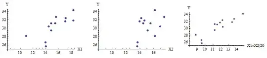
(Correlation is a useful way to describe these relationships because all three plots appear sufficiently linear and homoscedastic.)

Let's do some regression.

1. Y ~ X1*X2. The p-value is 0.000072 and the mean square residual is 1.37.

2. Y ~ X1 + X2. The p-values are .00041 and .00038, respectively. The mean square residual is 1.33. The individual p-values are not as low as in the preceding model (if you care about such things) and the mean square residual is only a tiny bit lower, despite using two variables instead of 1.

3. Y ~ X1 + X2 + X1*X2. The p-values are .00033, .0028, and 0.129, respectively. The interaction (X1*X2) is not significant. (The mean square error has improved to 1.098, though.)

This perfectly conforms to the description of the problem: the significance of the interaction goes away when accompanied by X1 and X2 in the model.

What is going on? I generated these data by drawing X1 and X2 independently from a Normal(15,2) distribution and then forming Y by adding Normal(0,1) error to X1 + X2. In other words, apart from that error, Y depends linearly on X1 and X2; there is no interaction.

We can understand this geometrically: the plot of a surface of the form $Y = \alpha X_1 + \beta X_2$, for positive $\alpha, \beta, X_1, X_2$, is a plane; the plot of a surface of the form $Y = \gamma X_1 X_2$ ($\gamma$ positive) is a very flat hyperboloid of one sheet, assuming $X_1$ and $X_2$ stay away from $0$. That hyperboloid can be a more than adequate approximation to the plane (first regression) which in turn might be a better model for $Y$.

As others have explained at length in the referenced thread, it is rare that you can interpret an interaction by itself (regression 1); you need to include it in the context of the linear terms (regression 3) or formulate a different model altogether (as described in my reply in the referenced thread).

Answer 2

The problem which arises is an issue of interpretation. Consider a simple linear regression model with a continuous main effect and continuous outcome. Suppose further you have a binary factor and you're interested in the model with interaction. When you adjust for the lower level terms, the interaction parameter has a meaningful definition: it is interpreted as the difference in slopes between regression lines between groups defined by the binary indicator.

When the lower level terms are dropped, there is no such interpretation. The quantity estimated has no physical meaning. It imposes the constraint that the two regression lines share the same intercept, but have different slopes. Putting such constraints on intercepts is ill-advised. As a parameter, the no-main-effects interaction term is strictly distinct from the orthodox parameter which has the main effects.

To answer your question, the X1:X2 terms in your two different model specifications are estimating two completely different parameters. It shouldn't be surprising to us that one is estimated to be significant and the other isn't, consequently.

Answer 3

I remember having read an very interesting article on this topic. I am very sorry not to be able to link it but the message was that interaction terms between two variables say $x_1$ and $x_2$ must have all three terms:

$y = \beta_0 +\beta_1x_1 + \beta_2x_2 + \beta_3x_1 \times x_2$

however, otherwise you may well run into omitted variable bias problems. In the meantime this may help you a bit: Understanding Interaction Models