I've been reading about generalised additive models. I've been using this data (which is a reformatted version of data from Hastie's website), and running my code in R. This data essentially consists of whether a patient has or does not have coronary heart disease (the variable to be modelled) and several patient characteristics. For the sake of this question, the two I am interested in are sbp (sytolic blood pressure) and chol.ratio (the ratio of two types of cholesterol). I've been trying to model chd with logistic regression.
Looking at scatterplots sbp seems non-linearly related to the logit, so I've modelled it with splines as follows:
Using gam:
data1 <- read.csv("coris.csv", sep = ",", stringsAsFactors = F,
                            header = T)
require(gam)
gam.object <- gam(chd ~ s(sbp, 5) + chol.ratio, data = data1,
                          family = binomial(link = "logit"))
And using the Design package:
require(design)
rcs.object <- lrm(chd ~ rcs(sbp, 6) + chol.ratio, data = data1)
I can plot the subsequent models in 3d using the rcl() package, and the outputs are very similar - the model using GAM is:
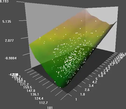
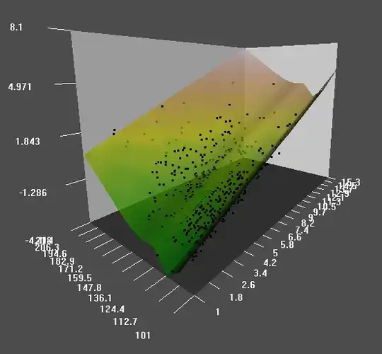
The plane represents the fitted model over a range of the predictor variables, and the points are the actual fitted model, the z axis to the right is the cholesterol ratio, and the x axis to the left is the sytolic blood pressure, and the vertical axis is the logit.
and the model using lrm with a rcs is :
So - with the lrm command are you actually fitting a generalized additive model if you specify a spline with rcs()? If not, why not, and how do the two approaches differ?