Your data
Looking at your data, I notice (a) that some days are missing, such as 2015-10-07 to 2015-10-10, and (b) that you do not have zero sales values. This looks very much as if your data contained only "actual" (that is, non-zero) transactions.
If so, the first step should be to edit your data so days with zero sales actually are included as zeros. (If you only include nonzero sales, you will be modeling sales conditional on being nonzero, so your forecast will be biased upward.)
Stationarity and non
Now that you have zeros in your data, taking logarithms as Qin suggests will not be possible any more. I'd recommend a different approach to tackling non-stationarity, anyway.
Stationarity essentially means that the data-generating process does not change over time. Thus, non-stationarity means that the DGP does change. Of course, the DGP can change over time in many different ways: there can be periodic seasonality, there can be trends, or there could even be changes in variance, while the expectation stays constant over time. It is important to figure out just how your time series is non-stationary, and how to deal with the specific type of non-stationarity involved.
With daily sales data, you usually have multiple seasonalities: one year-over-year, and one within weeks. (People do more shopping on Saturday.) Or even monthly or biweekly seasonality, based on when paychecks arrive. Your variance will usually also be higher on the weekend. Long-range trends are usually not overly important, but you may have lifecycle effects, e.g., in fashion or consumer electronics. In addition, you may have causal effects like promotions, price changes or markdowns. To be honest, once these effects are taken care of, my impression is that there are few additional autoregressive or moving average dynamics left to model.
Finally, you appear to have very fine-grained data, on store level? Your data appears to be all integers, that is, count data.
ARIMA for sales data (or not)
Now, ARIMA may not be your best choice. First, it is not built for count data series - ARIMA models expect normally distributed errors. There are a few Integer ARMA (INARMA) models around, but these are not very common.
In addition, ARIMA or INARMA cannot deal with multiple seasonalities, as you probably have in your data. You could simply work with frequency=7 to pick up the weekly seasonality, disregard the yearly seasonality, and hope for the best. (If you have less than two years of data, you won't be able to make ARIMA fit yearly seasonality, anyway.)
(EDIT) Finally, you have a nine-month period where the product apparently was not available at all. ARIMA cannot deal with this. If you apply ARIMA to a time series such as this, you will either need to fill in the entire nine months with zeros (which would simulate true zero demand - but if the product was unavailable, we don't know demand during this period, so filling zeros is unwarranted), or you'd just disregard the hole and "squash" your data together - even though sales in January may have very little to do with those in October. Both are obviously inappropriate.
Recommendations
My recommendation would be to run a count data model, say a Poisson regression or a negative binomial regression, using day-of-week dummies and some kind of hump functions for yearly seasonality (if you have at least one year of history). Add any promotional campaigns you know of as regressors.
If you don't have any promotional campaigns, you could also try a very simple benchmark: for next Monday, forecast average sales over historical Mondays; for next Tuesday, forecast average sales over historical Tuesdays, and so forth. This looks very naive, but it performed extremely well in a paper I have recently had accepted in the International Journal of Forecasting (Kolassa, 2016).
Forecast evaluation
Whatever you do, make sure to evaluate your forecasts using appropriate criteria - that is, some kind of Mean Squared Error (MSE). Do not use the Mean Absolute Error (MAE) for skewed count data - if you minimize the MAE, you will get forecasts that are biased. In extreme cases (say, Poisson distributed sales with a mean below $\log 2\approx 0.69$), your MAE will be lowest for a flat zero forecast. See here and here for details.
Further reading
Here is an older related answer of mine. And here is a free online forecasting textbook I'd recommend.
In R
Let's run this through R. Here is your data:
dataset <- structure(list(
  date = structure(c(16436, 16437, 16438, 16439, 16440, 16713, 16714,
    16719, 16722, 16725, 16726, 16729, 16732, 16733, 16734, 16736,
    16739, 16741, 16742, 16744, 16745, 16746, 16749, 16753, 16755,
    16756, 16757, 16761, 16762, 16765, 16766, 16768), class = "Date"),
  sales = c(2, 1, 3, 3, 2, 1, 1, 1, 1, 2, 1, 1, 1, 2, 1, 1, 2, 1, 1,
    1, 1, 1, 2, 3, 1, 1, 1, 3, 3, 3, 2, 4)),
  .Names = c("date", "sales"), row.names = c(NA, -32L), class = "data.frame")
(I read it in using scan(), then created this reproducible example using dput(). You can read your data from a file using read.table().)
Let's plot this. Always start by plotting the data:
with(dataset,plot(date,sales,type="o",pch=19,xlab="",ylab="",
  ylim=range(c(0,dataset$sales))))
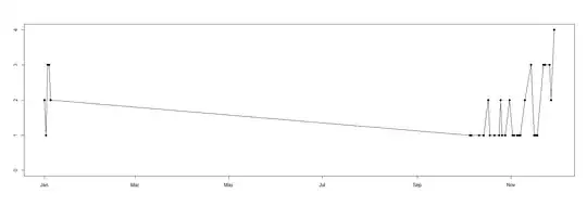
Now, you write in your comment that your data is seasonal. That explains the long string of no data between 2015-01-05 and 2015-10-05. However, you have positive sales on 2015-10-05, 06, 11 and 14. In my experience, this means that product was available on 2015-10-07, 08, 09, 10, 12 and 13, but that there simply was zero demand. As per above, we need to take these zero demands into account in modeling and forecasting, since zero demands will occur again in the future, and if we don't consider them historically, our forecasts will be biased upward. So I'll transform your data by filling in zeros on dates with no sales records between 2015-10-05 and 2015-11-29. (I would do the same between 2015-01-01 and 2015-01-05, but all dates there do have nonzero sales records.)
(Note incidentally, that we have a source of potential confusion here. To a retailer, a "seasonal" product is often one that is only available during certain times of the year. To the time series analyst and forecaster, "seasonal" is a time series that is defined the entire time, but exhibits seasonal peaks and troughs.)
dataset.new <- data.frame(
  date=seq(min(dataset$date),max(dataset$date),by="day"),sales=NA)
dataset.new[as.Date("2015-10-05")<=dataset.new$date,"sales"] <- 0
dataset.new[dataset.new$date %in% dataset$date,"sales"] <- dataset$sales
(Note that the last line relies on both dataset and dataset.new being sorted by date.)
with(dataset.new,plot(date,sales,type="o",pch=19,xlab="",ylab=""))
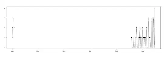
Note the zero sales inferred at the end.
Now we can start modeling. Let's first define a forecast period:
horizon <- 30
dates.forecast <- max(dataset.new$date)+(1:horizon)
We start with a simple day-of-week model, which will simply forecast the average of Monday sales for future Mondays and so forth, as proposed above. The easiest way to do this is to use lm() to create a linear model together with weekdays():
model.dow <- lm(sales~weekdays(date)-1,dataset.new)
summary(model.dow)
forecast.dow <- predict(model.dow,newdata=data.frame(date=dates.forecast))
The summary shows the inner workings of the model. Here is part of its output:
Coefficients:
                        Estimate Std. Error t value Pr(>|t|)
weekdays(date)Friday      0.4444     0.3464   1.283 0.204969
weekdays(date)Monday      1.0000     0.3464   2.887 0.005586 **
weekdays(date)Saturday    1.3333     0.3464   3.849 0.000316 ***
weekdays(date)Sunday      1.5556     0.3464   4.491 3.78e-05 ***
weekdays(date)Thursday    0.6667     0.3464   1.925 0.059566 .
weekdays(date)Tuesday     0.6250     0.3674   1.701 0.094687 .
weekdays(date)Wednesday   0.5000     0.3674   1.361 0.179219
Since I used -1 in my lm() call, no intercept is used, so the coefficients correspond to the weekday averages and the forecasts.
We can also add a trend, simply by adding a +date in the lm() formula, since dates are internally converted to counts of days:
model.dow.trend <- lm(sales~weekdays(date)+date-1,dataset.new)
summary(model.dow.trend)
forecast.dow.trend <- predict(model.dow.trend,newdata=data.frame(date=dates.forecast))
Here is the summary:
Coefficients:
                         Estimate Std. Error t value Pr(>|t|)
weekdays(date)Friday    61.722324  25.609466   2.410   0.0194 *
weekdays(date)Monday    62.266061  25.604528   2.432   0.0184 *
weekdays(date)Saturday  62.614880  25.610999   2.445   0.0178 *
weekdays(date)Sunday    62.840770  25.612531   2.454   0.0175 *
weekdays(date)Thursday  61.940878  25.607933   2.419   0.0190 *
weekdays(date)Tuesday   62.015965  25.656988   2.417   0.0191 *
weekdays(date)Wednesday 61.894633  25.658521   2.412   0.0193 *
date                    -0.003668   0.001533  -2.393   0.0203 *
The date coefficient tells us that sales decrease by 0.0037 units per day. (Remember that there were quite a few inferred zero sales dates near the end of your time series, but none at the beginning.)
Let's plot:
with(dataset.new,plot(date,sales,type="o",pch=19,xlab="",ylab="",
    xlim=range(c(dataset.new$date,dates.forecast))))
lines(dates.forecast,forecast.dow,type="o",pch=19,col="red")
lines(dates.forecast,forecast.dow.trend,type="o",pch=19,col="green")

We can see the day-of-week pattern, as well as the downward trend in the green forecast. If you want longer-range trended forecasts, it is good practice to dampen the trend, for which you'd need to explicitly define a trend column in your data matrices.
Now you can also start including hump function as additional data matrix columns, in order to model seasonal patterns (in the time series sense, see above). However, with the little data you have, I'd be very careful about creating too complex a model - your forecast accuracy will likely go down soon as you start overfitting.


