What I usually use as the measure of reconstruction error (in the context of PCA, but also other methods) is the coefficient of determination $R^2$ and the Root Mean Squared Error (or normalised RMSE). These two are easy to compute and give you a quick idea of what the reconstruction did.
Calculation
Let's assume $X$ is your original data and $f$ is the compressed data.
The $R^2$ of the $i^{th}$ variable can be computed as:
$R^2_i = 1 - \frac{\sum_{j=1}^n (X_{j,i} - f_{j,i})^2}{\sum_{j=1}^n X_{j,i}^2}$
Since $R^2 = 1.0$ for a perfect fit, you can judge the reconstruction by how close the $R^2$ is to 1.0.
The RMSE of the $i^{th}$ variable can be computed as:
$
\text{RMSE}_i = \sqrt{\overline{(X_i - f_i)^2}}
$
which you can also normalise by a quantity that suits you (norm $N$), I often normalise by the mean value, the NRMSE is thus:
$\text{NRMSE}_i = \frac{\text{RMSE}_i}{N_i} = \sqrt{\frac{\overline{(X_i - f_i)^2}}{\overline{X_i^2}}}$
Computation
In case you are using Python you can compute these as:
from sklearn.metrics import r2_score
from sklearn.metrics import mean_squared_error
from math import sqrt
import numpy as np

r2 = r2_score(X, f)
rmse = sqrt(mean_squared_error(X, f))

# RMSE normalised by mean:
nrmse = rmse/sqrt(np.mean(X**2))
where X is the original data and f is the compressed data.
Visualization
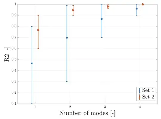
In case it is helpful for you to do some sensitivity analysis you can then judge visually how the $R^2$ or RMSE change when you change parameters of your compression. For instance, this can be handy in the context of PCA when you want to compare reconstructions with increasing number of the retained Principal Components. Below you see that increasing the number of modes is getting your fit closer to the model: