How to compare 2 non-stationary time series to determine a correlation?

Question

I have two data series that plot median age at death over time. Both series demonstrate an increased age at death over time, but one much lower than another. I want to determine if the increase in the age at death of the lower sample is significantly different than that of the upper sample.

Here are the data, ordered by year (from 1972 through 2009 inclusive) as rounded to three decimal places:

Cohort A    70.257  70.424  70.650  70.938  71.207  71.263  71.467  71.763  71.982  72.270  72.617  72.798  72.964  73.397  73.518  73.606  73.905  74.343  74.330  74.565  74.558  74.813  74.773  75.178  75.406  75.708  75.900  76.152  76.312  76.558  76.796  77.057  77.125  77.328  77.431  77.656  77.884  77.983
Cohort B    5.139   8.261   6.094   12.353  11.974  11.364  12.639  11.667  14.286  12.794  12.250  14.079  17.917  16.250  17.321  18.182  17.500  20.000  18.824  21.522  21.500  21.167  21.818  22.895  23.214  24.167  26.250  24.375  27.143  24.500  23.676  25.179  24.861  26.875  27.143  27.045  28.500  29.318

Both series are non-stationary - how can I compare the two please? I'm using STATA. Any advice would be gratefully received.

Answer 1

This is a simple situation; let's keep it so. The key is to focus on what matters:

• Obtaining a useful description of the data.

• Assessing individual deviations from that description.

• Assessing the possible role and influence of chance in the interpretation.

• Maintaining intellectual integrity and transparency.

There are still many choices and many forms of analysis will be valid and effective. Let's illustrate one approach here that can be recommended for its adherence to these key principles.

To maintain integrity, let's split the data into halves: the observations from 1972 through 1990 and those from 1991 through 2009 (19 years in each). We will fit models to the first half and then see how well the fits work in projecting the second half. This has the added advantage of detecting significant changes that may have occurred during the second half.

To obtain a useful description, we need to (a) find a way to measure the changes and (b) fit the simplest possible model appropriate for those changes, evaluate it, and iteratively fit more complex ones to accommodate deviations from the simple models.

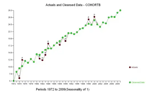
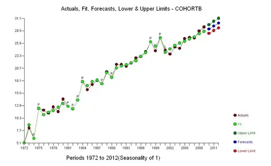
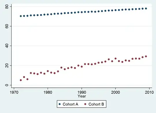
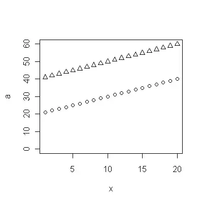
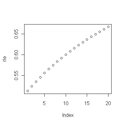
(a) You have many choices: you can look at the raw data; you can look at their annual differences; you can do the same with the logarithms (to assess relative changes); you can assess years of life lost or relative life expectancy (RLE); or many other things. After some thought, I decided to consider RLE, defined as the ratio of life expectancy in Cohort B relative to that of the (reference) Cohort A. Fortunately, as the graphs show, the life expectancy in Cohort A is increasing regularly in a stable fashion over time, so that most of the random-looking variation in the RLE will be due to changes in Cohort B.

(b) The simplest possible model to start with is a linear trend. Let's see how well it works.

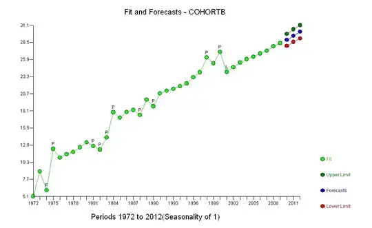
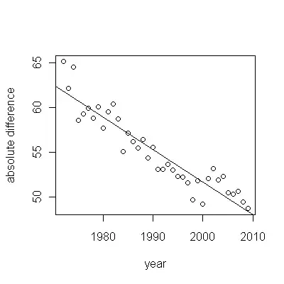
The dark blue points in this plot are the data retained for fitting; the light gold points are the subsequent data, not used for the fit. The black line is the fit, with a slope of .009/year. The dashed lines are prediction intervals for individual future values.

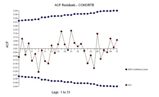
Overall, the fit looks good: examination of residuals (see below) shows no important changes in their sizes over time (during the data period 1972-1990). (There is some indication that they tended to be larger early on, when life expectancies were low. We could handle this complication by sacrificing some simplicity, but the benefits for estimating the trend are unlikely to be great.) There is just the tiniest hint of serial correlation (exhibited by some runs of positive and runs of negative residuals), but clearly this is unimportant. There are no outliers, which would be indicated by points beyond the prediction bands.

The one surprise is that in 2001 the values suddenly fell to the lower prediction band and stayed there: something rather sudden and large happened and persisted.

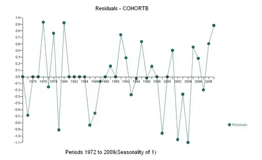
Here are the residuals, which are the deviations from the description mentioned previously.

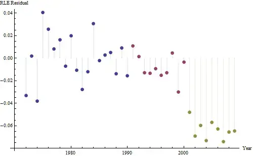
Because we want to compare the residuals to 0, vertical lines are drawn to the zero level as a visual aid. Again, the blue points show data used for the fit. The light gold ones are the residuals for data falling near the lower prediction limit, post-2000.

From this figure we can estimate that the effect of the 2000-2001 change was about -0.07. This reflects a sudden drop of 0.07 (7%) of a full lifetime within Cohort B. After that drop, the horizontal pattern of residuals shows that the previous trend continued, but at the new lower level. This part of the analysis should be considered exploratory: it was not specifically planned, but came about due to a surprising comparison between the held-out data (1991-2009) and the fit to the rest of the data.

One other thing--even using just the 19 earliest years of data, the standard error of the slope is small: it's only .0009, just one-tenth of the estimated value of .009. The corresponding t-statistic of 10, with 17 degrees of freedom, is extremely significant (the p-value is less than $10^{-7}$); that is, we can be confident the trend is not due to chance. This is one part of our assessment of the role of chance in the analysis. The other parts are the examinations of the residuals.

There appears to be no reason to fit a more complicated model to these data, at least not for the purpose of estimating whether there's a genuine trend in RLE over time: there is one. We could go further and split the data into pre-2001 values and post-2000 values in order to refine our estimates of the trends, but it wouldn't be completely honest to conduct hypothesis tests. The p-values would be artificially low, because the splitting testing were not planned in advance. But as an exploratory exercise, such estimation is fine. Learn all you can from your data! Just be careful not to deceive yourself with overfitting (which is almost sure to happen if you use more than a half dozen parameters or so or use automated fitting techniques), or data snooping: stay alert to the difference between formal confirmation and informal (but valuable) data exploration.

Let's summarize:

• By selecting an appropriate measure of life expectancy (the RLE), holding out half the data, fitting a simple model, and testing that model against the remaining data, we have established with high confidence that: there was a consistent trend; it has been close to linear over a long period of time; and there was a sudden persistent drop in RLE in 2001.

• Our model is strikingly parsimonious: it requires just two numbers (a slope and intercept) to describe the early data accurately. It needs a third (the date of the break, 2001) to describe an obvious but unexpected departure from this description. There are no outliers relative to this three-parameter description. The model is not going to be substantially improved by characterizing serial correlation (the focus of time-series techniques generally), attempting to describe the small individual deviations (residuals) exhibited, or introducing more complicated fits (such as adding in a quadratic time component or modeling changes in the sizes of the residuals over time).

• The trend has been 0.009 RLE per year. This means that with each passing year, the life expectancy within Cohort B has had 0.009 (almost 1%) of a full expected normal lifetime added to it. Over the course of the study (37 years), that would amount to 37*0.009 = 0.34 = one-third of a full lifetime improvement. The setback in 2001 reduced that gain to about 0.28 of a full lifetime from 1972 to 2009 (even though during that period overall life expectancy increased 10%).

• Although this model could be improved, it would likely need more parameters and the improvement is unlikely to be great (as the near-random behavior of the residuals attests). On whole, then, we should be content to arrive at such a compact, useful, simple description of the data for so little analytical work.

Answer 2

I think that whuber's answer is straightforward and a simple one for a non-time series person like me to understand. I base mine on his. My answer is in R not Stata as I don't know stata that well.

I wonder if the question is actually asking us to look at whether the absolute year on year increase is the same in the two cohorts (rather than relative). I think this is important and illustrate it as follows. Consider the following toy example:

a <- 21:40
b <- 41:60
x <- 1:20
plot(y = a, x = x, ylim = c(0, 60))
points(y = b, x = x, pch = 2)

Here we have 2 cohorts, each of which have a steady 1 year per year increase in median survival. So each year both cohorts in this example increase by the same absolute amount, but the RLE gives the following:

rle <-  a / b
plot(rle)

Which obviously has an upward trend, and the p value to test the hypothesis that the gradient of the line 0 is 2.2e-16. The fitted straight line (let's ignore that this line looks curved) has a gradient of 0.008. So even though both cohorts have the same absolute increase in a year, the RLE has an upward slope.

So if you use RLE when you want to look for absolute increases, then you'll inappropriately reject the null hypothesis.

Using the supplied data, calculating the absolute difference between the cohorts we get:

Which implies that the absolute difference between median survival is gradually decreasing (i.e. the cohort with the poor survival is gradually getting closer to the cohort with the better survival).

Answer 3

These two time series seems to have a deterministic trend. This is one relation that you obviously want to remove before further analysis. Personally, i would proceed as follows:

1) I would run a regression for each time series against a constant and a time, and compute the residual for each time series.

2) Taking the two residuals series, computed in the step above, i would run a simple linear regression (without a constant term) and look at the t-statistic, p-value, and decided on whether or not there is further dependence between the two series.

This analysis assumes the same set of assumption you make in a linear regression.

Answer 4

In some cases one knows a theoretical model which can used to test your hypothesis. In my world tis "knowledge" is often absent and one must resort to statistical techniques that can be classified as exploratory data analysis which summarizes what follows.When analyzing time series data that are non-stationary i.e. has autocorrelative properties simple cross-correlation tests are often misleading insofar as false positives can be easily found. One of the earliest analysis of this is found in Yule, G.U, 1926, "Why do we sometimes get nonsense correlations between time series? A study in sampling and the nature of time series", Journal of the Royal Statistical Society 89, 1–64 . Alternatively when one or more of the series themselves have been effected by exceptional activity ( see whuber "the sudden setback in Cohort B at 2001 ) which can effectively hide significant relationships. Now detecting a relationship between time series extends to examining not only contemporaneous relationships but possible lagged relationships. Continuing, if either series has been effected by anomalies ( one-time events ) then we must robustify our analysis by adjusting for these one-time distortions. The literature of time series points out how to identify the relationship via pre-whitening in order to more clearly identify structure. Pre-whitening adjusts for intra-correlative structure prior to identifying inter-correlative structure. Notice the key word was identifying structure. This approach easily leads to the following "useful model" :

Y(T) = -194.45
+[X1(T)][(+ 1.2396+ 1.6523B** 1)] COHORTA

   +[X2(T)][(- 3.3924)]                :PULSE          3

   +[X3(T)][(- 2.4760)]                :LEVEL SHIFT   30 reflecting persistant  unusal activity

   +[X4(T)][(+ 1.1453)]                :PULSE         29

   +[X5(T)][(- 2.7249)]                :PULSE         11

   +[X6(T)][(+ 1.5248)]                :PULSE         27

   +[X7(T)][(+ 2.1361)]                :PULSE          4

   +[X8(T)][(+ 1.6395)]                :PULSE         13

   +[X9(T)][(- 1.6936)]                :PULSE         12

   +[X10(T)[(- 1.6996)]                :PULSE         19

   +[X11(T)[(- 1.2749)]                :PULSE         10

   +[X12(T)[(- 1.2790)]                :PULSE         17

  +       [A(T)]

which suggests a contemporary relationship of 1.2936 and a lagged effect of 1.6523. Note that there were a number of years where unusual activity was identified viz. (1975,2001,1983,1999,1976,1985,1984,1991 and 1989). The adjustments for the years allows us to more clearly assess the relationship between these two series.

In terms of making a forecast

MODEL EXPRESSED AS AN XARMAX
Y[t] = a[1]Y[t-1] + ... + a[p]Y[t-p]
+ w[0]X[t-0] + ... + w[r]X[t-r]
+ b[1]a[t-1] + ... + b[q]a[t-q]
+ constant

THE RIGHT-HAND SIDE CONSTANT IS: -194.45

COHORTA 0 1.239589 X( 39 ) * 78.228616 = 96.971340

COHORTA 1 1.652332 X( 38 ) * 77.983000 = 128.853835

I~L00030 0 -2.475963 X( 39 ) * 1.000000 = -2.475963

      NET PREDICTION FOR Y(    39 )=                     28.894826 

Four coefficients is all that is required to make a forecast and of course a prediction for CohortA at time period 39 (78.228616) obtained from the ARIMA model for Cohorta.

Answer 5

This answer containd some graphics