Expectation of a product of $n$ dependent random variables when $n\to\infty$

Question

Let $X_1 \sim U[0,1]$ and $X_i \sim U[X_{i - 1}, 1]$, $i = 2, 3,...$. What is the expectation of $X_1 X_2 \cdots X_n$ as $n \rightarrow \infty$?

Answer 1

The answer is indeed $1/e$, as guessed in the earlier replies based on simulations and finite approximations.

The solution is easily arrived at by introducing a sequence of functions $f_n: [0,1]\to[0,1]$. Although we could proceed to that step immediately, it might appear rather mysterious. The first part of this solution explains how one might cook up these $f_n(t)$. The second part shows how they are exploited to find a functional equation satisfied by the limiting function $f(t) = \lim_{n\to\infty}f_n(t)$. The third part displays the (routine) calculations needed to solve this functional equation.

---

1. Motivation

We can arrive at this by applying some standard mathematical problem-solving techniques. In this case, where some kind of operation is repeated ad infinitum, the limit will exist as a fixed point of that operation. The key, then, is to identify the operation.

The difficulty is that the move from $E[X_1X_2\cdots X_{n-1}]$ to $E[X_1X_2\cdots X_{n-1}X_n]$ looks complicated. It is simpler to view this step as arising from adjoining $X_1$ to the variables $(X_2, \ldots, X_n)$ rather than adjoining $X_n$ to the variables $(X_1, X_2, \ldots, X_{n-1})$. If we were to consider $(X_2, \ldots, X_n)$ as being constructed as described in the question--with $X_2$ uniformly distributed on $[0,1]$, $X_3$ conditionally uniformly distributed on $[X_2, 1]$, and so on--then introducing $X_1$ will cause every one of the subsequent $X_i$ to shrink by a factor of $1-X_1$ towards the upper limit $1$. This reasoning leads naturally to the following construction.

As a preliminary matter, since it's a little simpler to shrink numbers towards $0$ than towards $1$, let $Y_i = 1-X_i$. Thus, $Y_1$ is uniformly distributed in $[0,1]$ and $Y_{i+1}$ is uniformly distributed in $[0, Y_i]$ conditional on $(Y_1, Y_2, \ldots, Y_i)$ for all $i=1, 2, 3, \ldots.$ We are interested in two things:

1. The limiting value of $E[X_1X_2\cdots X_n]=E[(1-Y_1)(1-Y_2)\cdots(1-Y_n)]$.

2. How these values behave when shrinking all the $Y_i$ uniformly towards $0$: that is, by scaling them all by some common factor $t$, $0 \le t \le 1$.

To this end, define

$$f_n(t) = E[(1-tY_1)(1-tY_2)\cdots(1-tY_n)].$$

Clearly each $f_n$ is defined and continuous (infinitely differentiable, actually) for all real $t$. We will focus on their behavior for $t\in[0,1]$.

---

2. The Key Step

The following are obvious:

1. Each $f_n(t)$ is a monotonically decreasing function from $[0,1]$ to $[0,1]$.

2. $f_n(t) \gt f_{n+1}(t)$ for all $n$.

3. $f_n(0) = 1$ for all $n$.

4. $E(X_1X_2\cdots X_n) = f_n(1).$

These imply that $f(t) = \lim_{n\to\infty} f_n(t)$ exists for all $t\in[0,1]$ and $f(0)=1$.

Observe that, conditional on $Y_1$, the variable $Y_2/Y_1$ is uniform in $[0,1]$ and variables $Y_{i+1}/Y_1$ (conditional on all preceding variables) are uniform in $[0, Y_i/Y_1]$: that is, $(Y_2/Y_1, Y_3/Y_1, \ldots, Y_n/Y_1)$ satisfy precisely the conditions satisfied by $(Y_1, \ldots, Y_{n-1})$. Consequently

$$\eqalign{ f_n(t) &= E[(1-tY_1) E[(1-tY_2)\cdots(1-tY_n)\,|\, Y_1]] \\ &= E\left[(1-tY_1) E\left[\left(1 - tY_1 \frac{Y_2}{Y_1}\right)\cdots \left(1 - tY_1 \frac{Y_n}{Y_1}\right)\,|\, Y_1\right]\right] \\ &= E\left[(1-tY_1) f_{n-1}(tY_1)\right]. }$$

This is the recursive relationship we were looking for.

In the limit as $n\to \infty$ it must therefore be the case that for $Y$ uniformly distributed in $[0,1]$ independently of all the $Y_i$,

$$f(t) = E[(1 - tY)f(tY)]=\int_0^1 (1 - ty) f(ty) dy = \frac{1}{t}\int_0^t (1-x)f(x)dx.$$

That is, $f$ must be a fixed point of the functional $\mathcal{L}$ for which

$$\mathcal{L}[g](t) = \frac{1}{t}\int_0^t (1-x)g(x)dx.$$

---

3. Calculation of the Solution

Clear the fraction $1/t$ by multiplying both sides of the equation $f(t)=\mathcal{L}[f](t)$ by $t$. Because the right hand side is an integral, we may differentiate it with respect to $t$, giving

$$f(t) + tf'(t) = (1-t)f(t).$$

Equivalently, upon subtracting $f(t)$ and dividing both sides by $t$,

$$f'(t) = -f(t)$$

for $0 \lt t \le 1$. We may extend this by continuity to include $t=0$. With the initial condition (3) $f(0)=1$, the unique solution is

$$f(t) = e^{-t}.$$

Consequently, by (4), the limiting expectation of $X_1X_2\cdots X_n$ is $f(1)=e^{-1} = 1/e$, QED.

---

Because Mathematica appears to be a popular tool for studying this problem, here is Mathematica code to compute and plot $f_n$ for small $n$. The plot of $f_1, f_2, f_3, f_4$ displays rapid convergence to $e^{-t}$ (shown as the black graph).

a = 0 <= t <= 1;
l[g_] := Function[{t}, (1/t) Integrate[(1 - x) g[x], {x, 0, t}, Assumptions -> a]];
f = Evaluate@Through[NestList[l, 1 - #/2 &, 3][t]]
Plot[f, {t,0,1}]

Answer 2

Update

I think it's a safe bet that the answer is $1/e$. I ran the integrals for the expected value from $n=2$ to $n=100$ using Mathematica and with $n=100$ I got

0.367879441171442321595523770161567628159853507344458757185018968311538556667710938369307469618599737077005261635286940285462842065735614

(to 100 decimal places). The reciprocal of that value is

2.718281828459045235360287471351873636852026081893477137766637293458245150821149822195768231483133554

The difference with that reciprocal and $e$ is

-7.88860905221011806482437200330334265831479532397772375613947042032873*10^-31

I think that's too close, dare I say, to be a rational coincidence.

The Mathematica code follows:

Do[
 x = Table[ToExpression["x" <> ToString[i]], {i, n}];
 integrand = Expand[Simplify[(x[[n - 1]]/(1 - x[[n - 1]])) 
Integrate[x[[n]], {x[[n]], x[[n - 1]], 1}]]];
 Do[
   integrand = Expand[Simplify[x[[i - 1]] 
 Integrate[integrand, {x[[i]], x[[i - 1]], 1}]/(1 - x[[i - 
     1]])]],
   {i, n - 1, 2, -1}]
  Print[{n, N[Integrate[integrand, {x1, 0, 1}], 100]}],
 {n, 2, 100}]

End of update

This is more of an extended comment than an answer.

If we go a brute force route by determining the expected value for several values of $n$, maybe someone will recognize a pattern and then be able to take a limit.

For $n=5$, we have the expected value of the product being

$$\mu_n=\int _0^1\int _{x_1}^1\int _{x_2}^1\int _{x_3}^1\int _{x_4}^1\frac{x_1 x_2 x_3 x_4 x_5}{(1-x_1) (1-x_2) (1-x_3) (1-x_4)}dx_5 dx_4 dx_3 dx_2 dx_1$$

which is 96547/259200 or approximately 0.3724807098765432.

If we drop the integral from 0 to 1, we have a polynomial in $x_1$ with the following results for $n=1$ to $n=6$ (and I've dropped the subscript to make things a bit easier to read):

$x$

$(x + x^2)/2$

$(5x + 5x^2 + 2x^3)/12$

$(28x + 28x^2 + 13x^3 + 3x^4)/72$

$(1631x + 1631x^2 + 791x^3 + 231x^4 + 36x^5)/4320$

$(96547x + 96547x^2 + 47617x^3 + 14997x^4 + 3132x^5 + 360x^6)/259200$

If someone recognizes the form of the integer coefficients, then maybe a limit as $n\rightarrow\infty$ can be determined (after performing the integration from 0 to 1 that was removed to show the underlying polynomial).

Answer 3

Nice question. Just as a quick comment, I would note that:

• $X_n$ will converge to 1 rapidly, so for Monte Carlo checking, setting $n = 1000$ will more than do the trick.

• If $Z_n = X_1 X_2 \dots X_n$, then by Monte Carlo simulation, as $n \rightarrow \infty$, $E[Z_n] \approx 0.367$.

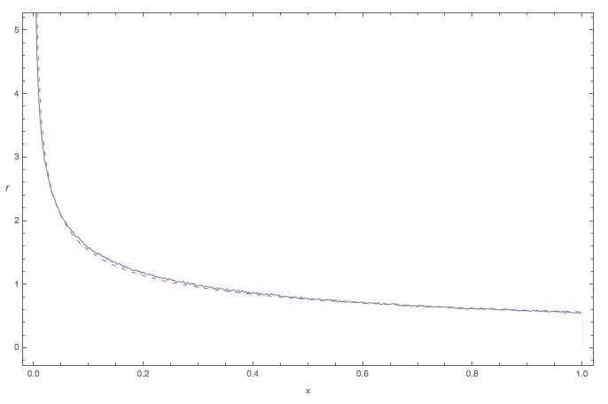
• The following diagram compares the simulated Monte Carlo pdf of $Z_n$ to a Power Function distribution [ i.e. a Beta(a,1) pdf) ]

$$f(z) = a z^{a-1}$$

... here with parameter $a=0.57$:

_{(source: tri.org.au)}

where:

• the blue curve denotes the Monte Carlo 'empirical' pdf of $Z_n$
• the red dashed curve is a PowerFunction pdf.

The fit appears pretty good.

Code

Here are 1 million pseudorandom drawings of the product $Z_n$ (say with $n = 1000$), here using Mathematica:

    data = Table[Times @@ NestList[RandomReal[{#, 1}] &, 
            RandomReal[], 1000], {10^6}];

The sample mean is:

     Mean[data]
> 0.367657  

Answer 4

Purely intuitively, and based on Rusty's other answer, I think the answer should be something like this:

    n = 1:1000
    x = (1 + (n^2 - 1)/(n^2)) / 2
    prod(x)

Which gives us 0.3583668. For each $X$, you are splitting the $(a,1)$ range in half, where $a$ starts out at $0$. So it's a product of $1/2, (1 + 3/4)/2, (1 + 8/9)/2$, etc.

This is just intuition.

---

The problem with Rusty's answer is that U[1] is identical in every single simulation. The simulations are not independent. A fix for this is easy. Move the line with U[1] = runif(1, 0, 1) to inside the first loop. The result is:

    set.seed(3)    #Just for reproducibility of my solution
    
    n = 1000    #Number of random variables
    S = 1000    #Number of Monte Carlo samples
    
    Z = rep(NA,S)
    U = rep(NA,n)
    
    for(j in 1:S){
        U[1] = runif(1,0,1)
        for(i in 2:n){
            U[i] = runif(1,U[i-1],1)
        }
        Z[j] = prod(U)
    }
    
    mean(Z)

This gives 0.3545284.