1

Is this a proper way to simulate the joint cdf of normal rvs with perfect positive correlation?

I followed these steps:

  1. I generate 10 000 observations for two independent uniform rvs, $U_1\sim U(0,1),U_2\sim U(0,1)$.

  2. The copula function for perfectly dependent rvs is the comonotonicity copula $C(u_1,u_2)=min(u_1,u_2)$. I plug in the simulated values of $U_1$ and $U_2$ to get simulated values of $C$.

  3. I transform $U_1$ and $U_2$ using the std. normal quantile function, to get $X_1\equiv \Phi^{-1}(U_1)$, $X_2\equiv \Phi^{-1}(U_2)$.

  4. I then gather together the simulated $(X_1,X_2,C)$. If I plot this triplet in a 3-dimensional plot, should it represent the cdf of bivariate normal variables with correlation coeff. 1?

Edit: This is not simulating from a Gaussian copula. This is about generating the cdf itself (the cdf depends on the marginal distributions).
p321
  • 11
  • 2
  • Are you sure about that? Notice step 4, where the value of $C$ depends on both $X_1$ and $X_2$. Also, the resulting cdf plot looks pretty much the same I get from plotting the bivariate normal cdf (included with the software). – p321 Dec 01 '15 at 15:24
  • This is not simulating FROM a Gaussian copula. This is simulating the values of the cdf. I believe they are completely different things? – p321 Dec 01 '15 at 15:28
  • I do want to simulate $F(X_1,X_2)$, so now we are on the right track. However, in order to simulate $F$ (its values), why would we need to generate dependent variables??? E.g. why not systematically go through each pair and look for the value of $F$? – p321 Dec 01 '15 at 15:39
  • 1
    @Xi'an is correct, because $C$ is nowhere used to generate $X_1$ and $X_2$. How about *you* try your approach and examine the scatterplot of $(X_1,X_2)$: I suspect it will help resolve some of the confusion that is present in steps 2-4. – whuber Dec 01 '15 at 15:40
  • The distribution of $F(X_1,X_2)$ obviously depend on the distribution of $(X_1,X_2)$. Hence, if you switch to another distribution for $(X_1,X_2)$, you obtain another distribution for $F(X_1,X_2)$. (_Addendum: A Normal pair with perfect correlation means that $X_1=X_2$ almost surely._) – Xi'an Dec 01 '15 at 15:41
  • I am not examining the scatterplot of (X_1,X_2). I plot the values of $F(X_1,X_2)$ in a 3-dimensional plot, because that's what I'm interested in. You are making me paranoid now O.o – p321 Dec 01 '15 at 15:42
  • Added a picture of the plot. – p321 Dec 01 '15 at 15:50
  • 1
    I think the initial sentence may be causing a lot of confusion. It asks how to "simulate" a "joint CDF." Later on, however, you cite the formula for the copula. It would therefore appear that nothing needs simulation. If you want to plot the CDF, why not do so directly? Simulation is used for *drawing random variables* from a given distribution. Thus it would seem you are asking for two entirely different things. What is your question, really? – whuber Dec 01 '15 at 15:51
  • 1
    How can I do so directly, if the marginals are not normal? That's the whole point of this simulation - visualizing the joint cdf with arbitrary marginals (and any kind of copula you would like). I assumed normal marginals only for simplicity and for easier comparison to the known cdf. – p321 Dec 01 '15 at 15:53
  • 3
    Thank you: that is a helpful comment. This post is attracting votes to close because many readers are interpreting it as a request for a way to simulate bivariate data from marginals and a copula (which has been answered at http://stats.stackexchange.com/questions/37424). Please, then, edit your question to emphasize that you are looking for ways to *visualize* a joint CDF based on its marginals and its copula function. – whuber Dec 01 '15 at 16:20
  • 2
    @whuber points out the fundamental difficulty with your formulation: you use a simulation terminology (simulate, generate) when you only want to visualise the 2d-cdf. – Xi'an Dec 01 '15 at 17:37

1 Answers1

3

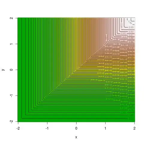
The joint cdf associated with the copula $\min(u_1,u_2)$ and Gaussian $\text{N}(0,1)$ marginals is $$F(x_1,x_2) = \min\{\Phi(x_1),\Phi(x_2)\}$$ which can be easily plotted. For instance,

x=y=seq(-2,2,le=123)
cog=matrix(0,123,123)
for (i in 1:123) for (j in 1:123) cog[i,j]=min(pnorm(x[i]),pnorm(y[j]))
image(x,y,cog,col=terrain.colors(50)
contour(x,y,cog,add=TRUE,nlevels=99)

produces the associated plot below with 1% level contours.

enter image description here

If you want the corresponding plot for another marginal $G$, just switch $G(X_i)$ for $\Phi(X_i)$.

Xi'an
  • 90,397
  • 9
  • 157
  • 575