20

I just noticed that integrating a univariate random variable's quantile function (inverse cdf) from p=0 to p=1 produces the variable's mean. I haven't heard of this relationship before now, so I'm wondering: Is this always the case? If so, is this relationship widely known?

Here is an example in python:

from math import sqrt
from scipy.integrate import quad
from scipy.special import erfinv

def normalPdf(x, mu, sigma):
    return 1.0 / sqrt(2.0 * pi * sigma**2.0) * exp(-(x - mu)**2.0 / (2.0 * sigma**2.0))

def normalQf(p, mu, sigma):
    return mu + sigma * sqrt(2.0) * erfinv(2.0 * p - 1.0)

mu = 2.5
sigma = 1.3
quantileIntegral = quad(lambda p: quantile(p,mu,sigma), 0.0, 1.0)[0]
print quantileIntegral # Prints 2.5.
amoeba
  • 93,463
  • 28
  • 275
  • 317
Tyler Streeter
  • 1,035
  • 9
  • 21

5 Answers5

30

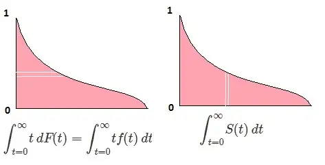
Let $F$ be the CDF of the random variable $X$, so the inverse CDF can be written $F^{-1}$. In your integral make the substitution $p = F(x)$, $dp = F'(x)dx = f(x)dx$ to obtain

$$\int_0^1F^{-1}(p)dp = \int_{-\infty}^{\infty}x f(x) dx = \mathbb{E}_F[X].$$

This is valid for continuous distributions. Care must be taken for other distributions because an inverse CDF hasn't a unique definition.

Edit

When the variable is not continuous, it does not have a distribution that is absolutely continuous with respect to Lebesgue measure, requiring care in the definition of the inverse CDF and care in computing integrals. Consider, for instance, the case of a discrete distribution. By definition, this is one whose CDF $F$ is a step function with steps of size $\Pr_F(x)$ at each possible value $x$.

Figure 1

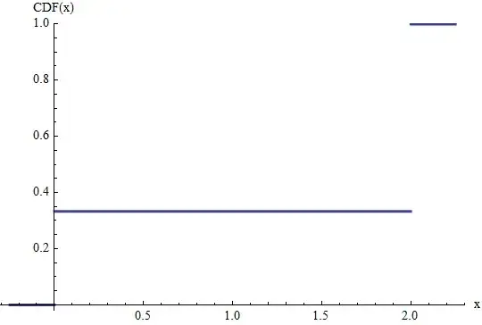
This figure shows the CDF of a Bernoulli$(2/3)$ distribution scaled by $2$. That is, the random variable has a probability $1/3$ of equalling $0$ and a probability of $2/3$ of equalling $2$. The heights of the jumps at $0$ and $2$ give their probabilities. The expectation of this variable evidently equals $0\times(1/3)+2\times(2/3)=4/3$.

We could define an "inverse CDF" $F^{-1}$ by requiring

$$F^{-1}(p) = x \text{ if } F(x) \ge p \text{ and } F(x^{-}) \lt p.$$

This means that $F^{-1}$ is also a step function. For any possible value $x$ of the random variable, $F^{-1}$ will attain the value $x$ over an interval of length $\Pr_F(x)$. Therefore its integral is obtained by summing the values $x\Pr_F(x)$, which is just the expectation.

Figure 2

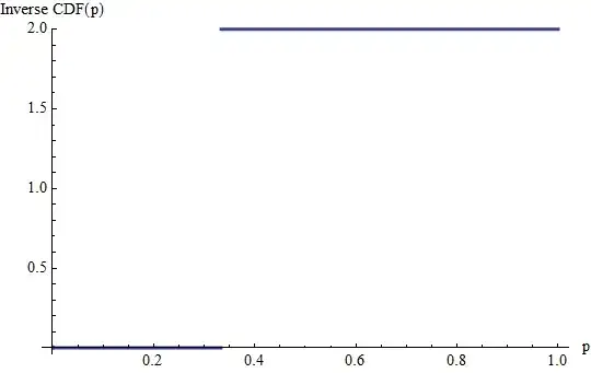
This is the graph of the inverse CDF of the preceding example. The jumps of $1/3$ and $2/3$ in the CDF become horizontal lines of these lengths at heights equal to $0$ and $2$, the values to whose probabilities they correspond. (The Inverse CDF is not defined beyond the interval $[0,1]$.) Its integral is the sum of two rectangles, one of height $0$ and base $1/3$, the other of height $2$ and base $2/3$, totaling $4/3$, as before.

In general, for a mixture of a continuous and a discrete distribution, we need to define the inverse CDF to parallel this construction: at each discrete jump of height $p$ we must form a horizontal line of length $p$ as given by the preceding formula.

whuber
  • 281,159
  • 54
  • 637
  • 1,101
  • 1
    you made a mistake in the change of variable. where does the x comes from? – Mascarpone Nov 15 '11 at 21:03
  • 3
    @Mascarpone Please read the text preceding the equation. I do not think there is a mistake in the change of variable :-), but if you think it would clarify the exposition, I would be happy to point out that when $p=F(x)$, then $x=F^{-1}(p)$. I just didn't think that was necessary. – whuber Nov 15 '11 at 21:04
  • now i got it ;), – Mascarpone Nov 15 '11 at 21:10
  • +1 Whuber: Thanks! Could you elaborate in order to use the formula you gave, how to take care for other distributions whose inverse CDF doesn't have a unique definition? – Tim Nov 26 '11 at 18:21
  • I added the elaboration you requested, @Tim. – whuber Nov 27 '11 at 16:33
  • 1
    To bypass such uneasy considerations about inverses, pseudo-inverses and the like, and simultaneously for a generalization to every moment, see [here](https://math.stackexchange.com/a/172857). – Did Nov 14 '18 at 09:04
  • 1
    @Did +1 Thank you for the elegant and memorable formulation. – whuber Nov 14 '18 at 15:03
10

An equivalent result is well known in survival analysis: the expected lifetime is $$\int_{t=0}^\infty S(t) \; dt$$ where the survival function is $S(t) = \Pr(T \gt t)$ measured from birth at $t=0$. (It can easily be extended to cover negative values of $t$.)

enter image description here

So we can rewrite this as $$\int_{t=0}^\infty (1-F(t)) \; dt$$ but this is $$\int_{q=0}^1 F^{-1}(q) \; dq$$ as shown in various reflections of the area in question

enter image description here

Henry
  • 30,848
  • 1
  • 63
  • 107
  • 2
    I like pictures, and instinctively feel there's a great idea lurking here--I *love* the idea--, but I don't understand these particular ones. Explanations would be helpful. One thing that stops me in my tracks is the thought of trying to extend the integral of $(1-F(t))dt$ to $-\infty$: it has to diverge. – whuber Nov 16 '11 at 04:14
  • @whuber: If you want to extend to negative $t$, you get $\int_{t=0}^\infty (1-F(t)) \; dt - \int_{t=-\infty}^0 F(t) \; dt$. Note that if this converges for a distribution symmetric about $0$, i.e. $F(t)=1-F(-t)$ then it is easy to see that the expectation is zero. Taking a sum rather than a difference $\int_{t=0}^\infty (1-F(t)) \; dt + \int_{t=-\infty}^0 F(t) \; dt$ gives the average absolute deviation about $0$. – Henry Nov 16 '11 at 08:01
  • If you like diagrams, you may be interested in this 1988 paper by Lee: [The Mathematics of Excess of Loss Coverages and Retrospective Rating-A Graphical Approach](http://casact.net/pubs/proceed/proceed88/88049.pdf). – Avraham Jun 19 '14 at 19:05
6

For any real-valued random variable $X$ with cdf $F$ it is well-known that $F^{-1}(U)$ has the same law than $X$ when $U$ is uniform on $(0,1)$. Therefore the expectation of $X$, whenever it exists, is the same as the expectation of $F^{-1}(U)$: $$E(X)=E(F^{-1}(U))=\int_0^1 F^{-1}(u)\mathrm{d}u.$$ The representation $X \sim F^{-1}(U)$ holds for a general cdf $F$, taking $F^{-1}$ to be the left-continuous inverse of $F$ in the case when $F$ it is not invertible.

Stéphane Laurent
  • 17,425
  • 5
  • 59
  • 101
4

We are evaluating:

enter image description here

Let's try with a simple change of variable:

enter image description here

And we notice that, by definition of PDF and CDF:

enter image description here

almost everywhere. Thus we have, by definition of expected value:

enter image description here

Mascarpone
  • 793
  • 1
  • 6
  • 7
1

Note that $F(x)$ is defined as $P(X\le x)$ and is a right-continuous function. $F^{-1}$ is defined as \begin{equation} F^{-1}(p)=\min(x|F(x)\ge p). \end{equation} The $\min$ makes sense because of the right continuity. Let $U$ be a uniform distribution on $[0, 1]$. You can easily verify that $F^{-1}(U)$ has the same CDF as $X$, which is $F$. This doesn't require $X$ to be continuous. Hence, $E(X)=E(F^{-1}(U))=\int_0^1F^{-1}(p)\mathop{dp}$. The integral is the Riemann–Stieltjes integral. The only assumption we need is the mean of $X$ exists ($E|X|<\infty$).

WWang
  • 41
  • 3