I am not necessarily interested in testing normality, but at least ensure that:
The mean is near 0
There is single mode
Tails are thinning out as you go further from the mean
Any ideas?
I am not necessarily interested in testing normality, but at least ensure that:
The mean is near 0
There is single mode
Tails are thinning out as you go further from the mean
Any ideas?
Distributions which satisfy those criteria can include distributions whose behavior is very different from the normal. For example, a $t$ distribution with two degrees of freedom satisfies those criteria, as does an asymmetric Laplace distribution, but each has very different properties from a normal.
I'll assume (though you don't state it) that you're primarily concerned with continuous variates. If you have discrete or even categorical data the advice would differ somewhat.
A common choice for assessing those sorts of things on data is the histogram, but caution is required; even small changes the binwidth and/or binorigin can in some cases lead to a big difference in appearance. Here's two histograms of the same data set:
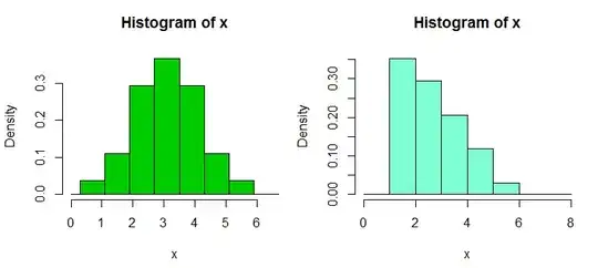
It's often advisable to use narrower bins than the common defaults packages offer; we're trying to get a visual idea of shape and can smooth by eye. [The smoothing of the default settings is often quite strong.]
Another alternative which can work well, particularly in large samples, is the kernel density estimate; again, you may want to use a bit less smoothing than the default by choosing a narrower bandwidth. Here's an example using the same data as above, but with half the default bandwidth, because the default (dashed curve) obscures the clumpiness in the original data that produce the inconsistency in the histogram:

This can sometimes be useful for spotting multiple modes, though small modes can be hard to spot (or tell apart from noise) with any dislay.
Another option is the quantile-quantile plot, or Q-Q plot - the normal Q-Q plot is very common - and this can convey a lot of information about shape, tail behavior (particularly if you want to see if tails are heavier than or lighter than that of a normal, say), and symmetry, but it takes some practice to learn to read them.

In this case the unusual both the suggestion of mild right skewness and the odd clumpiness can be seen. Judging symmetry can be aided by also displaying a density estimate for $2M-x$ (where $M$ is some measure of center, perhaps the median for example). You don't have to calculate a new density estimate for that; the original just needs to be plotted against $2M-x$ instead of $x$.