Neural net with hidden layer performing worse than without?

Question

I'm attempting to train a classifier on a single input vector of length 3000, and trying to predict which of 30 classes each input vector belongs to.

With 1M labeled input/output examples (split 80% training, 20% validate), I can get about 50% accuracy by simply training weights on a 3000 by 30 matrix. In other words, 50% accuracy with no hidden layer.

When I add a hidden layer with 100 neurons, or 500, or 50, I am consistently seeing worse performance than in my network with no hidden layers. I expect this is somehow a function of my hyperparameters, but I have tried tweaking the learning rate and batch size across a wide range of values. I've also tried sigmoid, tanh, and relu outputs on the hidden layer.

No matter what I try, I'm not seeing better than 20% accuracy when I add a hidden layer.

Happy to provide more detail as needed, but basically I'm looking for advice about how to debug (I'm using this as an excuse to explore Tensorflow.) I'd expect that my network with a hidden layer should at least as well as without.

---

Example code

Here is how I'm training the model (note that I've also tried sigmoid and tanh units, and adding a regularization term to my cost). The next_batch function creates a batch by randomly choosing a set of input/output pairs from a pool of about a million lableed examples. If I cut the hidden layer out altogether, it learns just fine.

HIDDEN_COUNT = 50

x = tf.placeholder("float", [None, FEATURE_COUNT])

Wh = init_weights((FEATURE_COUNT, HIDDEN_COUNT))
bh = tf.Variable(tf.zeros([HIDDEN_COUNT]))
h = tf.nn.relu(tf.matmul(x, Wh) + bh)

b = tf.Variable(tf.zeros([CATEGORY_COUNT]))
W = init_weights((HIDDEN_COUNT, CATEGORY_COUNT))
y = tf.nn.softmax(tf.matmul(h,W) + b)

y_ = tf.placeholder("float", [None,CATEGORY_COUNT])

cross_entropy = -tf.reduce_sum(y_*tf.log(y))
train_step = tf.train.GradientDescentOptimizer(.0001).minimize( cross_entropy )



# Test trained model
correct_prediction = tf.equal(tf.argmax(y,1), tf.argmax(y_,1))
accuracy = tf.reduce_sum(tf.cast(correct_prediction, "float"))

And then, inside a loop...

batch_xs, batch_ys = next_batch('train', batch_size)
train_step.run({x: batch_xs, y_: batch_ys})

Example output

Training on 500k examples, batched into 50-sample batches, with a test evaluation after every 200 batches:

accuracy: 0.031     cost: 71674 after 0 examples
accuracy: 0.187     cost: 70403 after 10000 examples
accuracy: 0.186     cost: 69147 after 20000 examples
accuracy: 0.187     cost: 68044 after 30000 examples
accuracy: 0.189     cost: 66978 after 40000 examples
accuracy: 0.192     cost: 65939 after 50000 examples
accuracy: 0.185     cost: 65112 after 60000 examples
accuracy: 0.187     cost: 64278 after 70000 examples
accuracy: 0.182     cost: 63690 after 80000 examples
accuracy: 0.185     cost: 62865 after 90000 examples
accuracy: 0.191     cost: 62023 after 100000 examples
accuracy: 0.186     cost: 61644 after 110000 examples
accuracy: 0.187     cost: 61155 after 120000 examples
accuracy: 0.189     cost: 60647 after 130000 examples
accuracy: 0.188     cost: 60209 after 140000 examples
accuracy: 0.187     cost: 59964 after 150000 examples
accuracy: 0.184     cost: 59496 after 160000 examples
accuracy: 0.186     cost: 59261 after 170000 examples
accuracy: 0.185     cost: 59127 after 180000 examples
accuracy: 0.186     cost: 58839 after 190000 examples
accuracy: 0.187     cost: 58884 after 200000 examples
accuracy: 0.184     cost: 58723 after 210000 examples
accuracy: 0.184     cost: 58493 after 220000 examples
accuracy: 0.189     cost: 58221 after 230000 examples
accuracy: 0.187     cost: 58176 after 240000 examples
accuracy: 0.189     cost: 58092 after 250000 examples
accuracy: 0.183     cost: 58057 after 260000 examples
accuracy: 0.184     cost: 58040 after 270000 examples
accuracy: 0.181     cost: 58369 after 280000 examples
accuracy: 0.189     cost: 57762 after 290000 examples
accuracy: 0.182     cost: 58186 after 300000 examples
accuracy: 0.189     cost: 57703 after 310000 examples
accuracy: 0.188     cost: 57521 after 320000 examples
accuracy: 0.185     cost: 57804 after 330000 examples
accuracy: 0.184     cost: 57883 after 340000 examples
accuracy: 0.184     cost: 57756 after 350000 examples
accuracy: 0.186     cost: 57505 after 360000 examples
accuracy: 0.185     cost: 57569 after 370000 examples
accuracy: 0.186     cost: 57562 after 380000 examples
accuracy: 0.204     cost: 57406 after 390000 examples
accuracy: 0.211     cost: 57432 after 400000 examples
accuracy: 0.185     cost: 57576 after 410000 examples
accuracy: 0.182     cost: 57774 after 420000 examples
accuracy: 0.183     cost: 57520 after 430000 examples
accuracy: 0.184     cost: 57421 after 440000 examples
accuracy: 0.186     cost: 57374 after 450000 examples
accuracy: 0.183     cost: 57552 after 460000 examples
accuracy: 0.186     cost: 57435 after 470000 examples
accuracy: 0.181     cost: 57210 after 480000 examples
accuracy: 0.182     cost: 57493 after 490000 examples

Note that attempting to lower the learning rate and resume after these 500k training samples produced no improvement in accuracy or cost.

Answer 1

Here are my thoughts on what could be going wrong:

Accuracy (what is being measured)

Perhaps your network is in fact doing well.

Let's consider binomial classification. If we have 50-50 distribution of labels, then 50% accuracy means the model is no better than chance (flipping a coin). If the Bernoulli distribution is 80%-20% and the accuracy is 50%, then the model is worse than chance.

No matter what I try, I'm not seeing better than 20% accuracy when I add a hidden layer.

If the accuracy is 20%, just negate the output and you have 80% accuracy, well done! (well at least for the binomial case).

Not so fast!

I believe that in your case the accuracy is misleading. This is a good read on the matter. For classification, the AUC (area under the curve) is often used. It's common to also examine the Receiver operating characteristic (ROC) and the confusion matrix.

For the multi-class case this becomes more tricky. Here is an answer that I found. Ultimately, this involves a strategy of 1-vs-rest or 1-vs-1 pairs, more on that here.

Pre-processing

• Are the features scaled? Do they have the same bounds? e.g [0,1]

• Have you tried standardizing the features? This renders each feature normally distributed with zero mean and unit variance.

• Perhaps normalization might help? Dividing each input vector by it's norm places it on the unit circle (for L2 norm) and also bounds the features (but scaling should be performed first otherwise the larger numbers will spike).

Training

As to the learning rate and momentum, if you're not in a big hurry, I would just set a low learning rate and the algorithm will converge better (although slower). This is valid for stochastic gradient descent where examples are shown at random (are you shuffling the data?). From your code I can't figure out how this happens. Are you going one pass only through the training data? For SGD, multiple iterations are made. Perhaps try smaller batches? Have you tried weight decay as a regularization method?

Architecture

Cross-entropy as loss function: check. Softmax at outputs: check.

Might be a longshot at this point but have you tried projection to a higher dimension in the first hidden layer then collapsing to a lower space in the next one two hidden layers?

There is also the cost in your output, I wonder if it could be scaled to make more sense. I would try to plot the evolution of the cost (log loss here) and see if it fluctuates or how steep it is. Your network might be stuck in a local minima plateau. Or it might be doing very well in which case double check the metric?

Hope this helped or generated some new ideas.

EDIT:

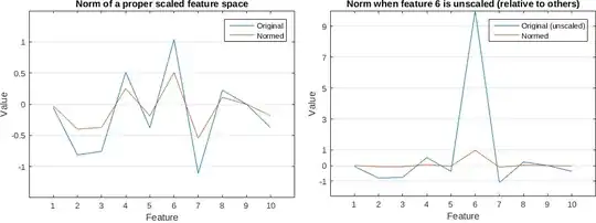
Example of how normalization (L2) can make things worse when features are not scaled relative to the other features. Plots for one sample:

In the left image the blue line is a vector of 10 values generated randomly with a mean zero and std of 1. In the right image I added an 'outlier' or out of scale feature no.6 where I set its value to 10. Clearly out of scale. When we normalize the out of scale vector, all other features become very close to 0 as it can be seen in the orange line on the right.

Standardizing the data might be a good thing to do before anything else in this case. Try plotting some histograms of the features or box plots.

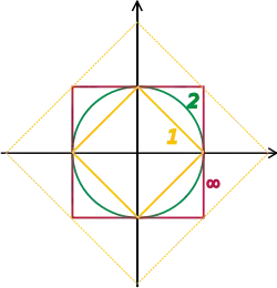
You mentioned you are normalizing the vectors to sum up to 1 and now it works better with 10. That means you are dividing by the 1-norm = sum(abs(X)) instead of the 2-norm (Euclidean) = sum(abs(X).^2)^(1/2). The L1 normalization generates sparser vectors, look at the figure below, where each axis is one feature, so this is a two dimensional space, however it can be generalized to an arbitrary number of dimensions.

Normalizing effectively places each vector on the edge of either shape. For L1 it will lie on the diamond somewhere. For L2 on the circle. When it hits the axis it is zero.