multivariate transformation of random variable

Question

Let $X$ and $Y$ be uniformly distributed over intervals $(-1, 1)$, and $(0, 1)$, respectively. Find the joint distribution of variables $U = XY$ and $V = Y$.

$X$ and $Y$ are independent.

I think it needs to be solved by finding the companion functions, inverting them, finding the Jacobian etc. etc., but I am not sure if I understand the problem correctly - the variables $U$ and $Y$ should be the companion functions? Or do I solve them separately? Thank you for any tips that you guys may have. Cheers

Answer 1

I have two suggestions:

1. Use differential algebra instead of Jacobians. It's a simpler, more reliable way to keep track of the derivatives.

2. Draw a picture. Often the trickiest part of such calculations is to determine what the domain of the new variables is. Pictures help.

Details and supporting code follow.

---

Two things need to be found: the probability element of $(U,V)$ and the domain (set of possible values) of $(U,V)$.

(The reason for choosing to write the distribution in terms of probability density, rather than a probability function, is that the probability function is somewhat messy to describe.)

The probability element

Using differential algebra it is straightforward to compute that

1. The probability element of the uniform distribution of $(X,Y)$ is $$f_{XY}(x,y)dx dy = \frac{1}{2}dx dy = \frac{1}{2}|dx\wedge dy|.$$

2. Computing the differentials of $u = xy$ and $v=y$, we easily obtain $$du = y\,dx + x\,dy;\ dv = dy,$$ whence $$du \wedge dv = (y\,dx + x\,dy)\wedge dy =y\,dx\wedge dy + x\,dy\wedge dy= y\,dx\wedge dy.$$

Comparing the two results, and recalling that $y = v$, shows immediately that

$$f_{UV}(u,v)du dv = \frac{1}{2v} |du \wedge dv| = \frac{1}{2v} du dv.$$

The domain

Since $-1 \le X \le 1$ and $0 \le Y \le 1$, it follows that

1. $0 \le Y = V \le 1$ and

2. $-1 \le X = U/V \le 1$, whence $|U| \le V.$

The transformation from $(X,Y)$ to $(U,V)$ can be visualized by drawing a large number of random values from $(X,Y)$ and coloring them according to $X$ and $Y$. The figure uses hue to represent $X$ and lightness to represent $Y$, with lighter points indicating smaller values of $Y$. On the left the points are plotted in $(X,Y)$ coordinates while on the right the same points are plotted in $(U,V)$ coordinates:

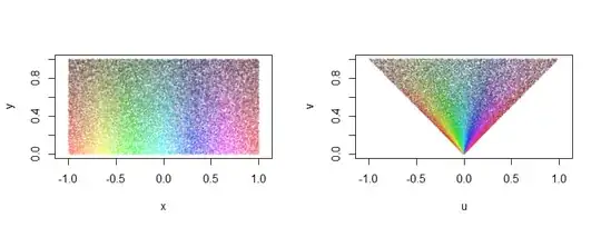
The points are squeezed towards the vertical axis, in proportion to their height above the horizontal axis. Each vertical line segment $X = x, 0 \le Y \le 1,$ is mapped to a radial line segment $V = \frac{1}{x}U, 0 \le V \le 1.$

Putting them together

Consequently, the probability density function for $(U,V)$ can be written in terms of indicator functions for its domain as

$$f_{UV}(u,v) = \frac{1}{2v} I(0 \le v \le 1) I(|u| \le v) du\,dv.$$

---

Code

As a check, we may integrate $f_{UV}$ over $\mathbb{R}^2$. It would be done in (say) Mathematica as

$$\int _{-\infty }^{\infty }\int _{-\infty }^{\infty }\frac{\text{Boole}[0\leq v\leq 1] \text{Boole}[\left| u\right| \leq v]}{2 v}dvdu$$

which, in response to this command, returns $1$ as the answer. Along with the evident fact that $f_{UV}$ is never negative, that verifies this actually is a probability density function.

The figure was drawn in R 3.1.3:

n <- 5e4
x <- runif(n, -1, 1)
y <- runif(n)
u <- x*y
v <- y
par(mfrow=c(1,2))
colors <- hsv((x+1)/2, .8, 1 - 0.8*y, .1)
plot(x, y, pch=16, col=colors, cex=3/8, asp=1)
plot(u, v, pch=16, col=colors, cex=1/4, asp=1)