Rotate PCA components to equalize the variance in each component

Question

I'm trying to reduce the dimensionality and noise of a dataset by performing PCA on the dataset and throwing away the last few PCs. After that, I want to use some machine learning algorithms on the remaining PCs, and therefore I want to normalize the data by equalizing the variance of the PCs to make the algorithms work better.

One simple way is to simply normalize the variance to unit values. However, the first PC contains more variance from the original dataset than the following ones, and I still want to give it more "weight". Therefore I was wondering: is there a simple way to just split its variance and share it with the PCs with less variances?

Another way is to map the PCs back to the original feature space, but in that case the dimensionality would also increase to the original value.

I guess it's better to keep the resultant columns orthogonal, but it's not necessary at this moment.

Answer 1

It is not completely clear to me that what you are asking is what you really need: a common preprocessing step in machine learning is dimensionality reduction + whitening, which means doing PCA and standardizing the components, nothing else. But I will nevertheless focus on your question as it is formulated, because it's more interesting.

---

Let $\mathbf X$ be the centered $n\times d$ data matrix with data points in rows and variables in columns. PCA amounts to singular value decomposition $$\mathbf X = \mathbf{USV}^\top \approx \mathbf U_k \mathbf S_k \mathbf V_k^\top,$$ where to perform the dimensionality reduction we keep only $k$ components. An orthogonal "factor rotation" of these components implies choosing an orthogonal $k \times k$ matrix $\mathbf R$ and plugging it into the decomposition: $$\mathbf X \approx \mathbf U_k \mathbf S_k \mathbf V_k^\top = \mathbf U_k \mathbf {RR}^\top \mathbf S_k \mathbf V_k^\top = \underbrace{\sqrt{n-1}\mathbf U_k^\phantom\top \mathbf {R}}_{\substack{\text{Rotated}\\\text{standardized scores}}} \cdot \underbrace{\mathbf R^\top \mathbf S_k \mathbf V_k^\top/\sqrt{n-1}}_{\text{Rotated loadings}^\top}.$$ Here $\sqrt{n-1}\mathbf U_k \mathbf R$ are rotated standardized components and the second term represents rotated loadings transposed. The variance of each component after rotation is given by the sum of squares of the corresponding loading vector; before rotation it is simply $s_i^2/(n-1)$. After rotation it is something else.

Now we are ready to formulate the problem in mathematical terms: given unrotated loadings $\mathbf L = \mathbf V_k \mathbf S_k / \sqrt{n-1}$, find rotation matrix $\mathbf R$ such that the rotated loadings, $\mathbf L \mathbf R$, has equal sum of squares in each column.

Let's solve it. Column sums of squares after rotation are equal to the diagonal elements of $$(\mathbf {LR})^\top \mathbf{LR} = \mathbf R^\top \frac{\mathbf S^2}{n-1} \mathbf R.$$ This makes sense: rotation simply redistributes the variances of components, which are originally given by $s_i^2/(n-1)$, between them, according to this formula. We need to redistribute them such they all become equal to their average value $\mu$.

I don't think there is a closed form solution to this, and in fact there are many different solutions. But a solution can be easily built in a sequential fashion:

1. Take the first component and the $k$-th component. The first one has variance $\sigma_\text{max}>\mu$ and the last one has the variance $\sigma_\text{min}<\mu$.
2. Rotate only these two such that the variance of the first becomes equal to $\mu$. Rotation matrix in 2D depends only on one parameter $\theta$ and it is easy to write down the equation and compute the necessary $\theta$. Indeed, $$\mathbf R_\text{2D} = \left(\begin{array}{cc}\cos \theta & \sin \theta \\ -\sin\theta & \cos \theta\end{array}\right)$$ and after transformation the first PC will get variance $$\cos^2\theta \cdot \sigma_\text{max} + \sin^2\theta \cdot \sigma_\text{min} = \cos^2\theta \cdot \sigma_\text{max} + (1-\cos^2\theta)\cdot \sigma_\text{min} =\mu,$$ from which we immediately obtain $$\cos^2\theta = \frac{\mu-\sigma_\text{min}}{\sigma_\text{max}-\sigma_\text{min}}.$$
3. The first component is now done, it has variance $\mu$.
4. Proceed to the next pair, taking the component with the largest variance and the one with the smallest variance. Goto #2.

This will redistribute all variances equally by a sequence of $(k-1)$ 2D rotations. Multiplying all these rotation matrices together will yield the overall $\mathbf R$.

---

Example

Consider the following $\mathbf S^2/(n-1)$ matrix: $$\left(\begin{array}{cccc}10&0&0&0\\0&6&0&0\\0&0&3&0\\0&0&0&1\end{array}\right).$$ The mean variance is $5$. My algorithm will proceed as follows:

1. Step 1: rotate PC1 and PC4 so that PC1 gets variance $5$. As a result, PC4 gets variance $1+(10-5)=6$.

2. Step 2: rotate PC2 (new maximal variance) and PC3 so that PC2 gets variance $5$. As a result, PC3 gets variance $3+(6-5)=4$.

3. Step 3: rotate PC4 (new maximal variance) and PC3 so that PC4 gets variance $5$. As a result, PC3 gets variance $4+(6-1)=5$.

4. Done.

I wrote the Matlab script that implements this algorithm (see below). For this input matrix, the sequence of rotation angles is:

48.1897   35.2644   45.0000

Component variances after each step (in rows):

10     6     3     1
 5     6     3     6
 5     5     4     6
 5     5     5     5

The final rotation matrix (product of three 2D rotation matrices):

 0.6667         0    0.5270    0.5270
      0    0.8165    0.4082   -0.4082
      0   -0.5774    0.5774   -0.5774
-0.7454         0    0.4714    0.4714

And the final $(\mathbf{LR})^\top \mathbf{LR}$ matrix is:

5.0000         0    3.1623    3.1623
     0    5.0000    1.0000   -1.0000
3.1623    1.0000    5.0000    1.0000
3.1623   -1.0000    1.0000    5.0000

Here is the code:

S = diag([10 6 3 1]);
mu = mean(diag(S));
R = eye(size(S));

vars(1,:) = diag(S);
Supdated = S;

for i = 1:size(S,1)-1
    [~, maxV] = max(diag(Supdated));
    [~, minV] = min(diag(Supdated));

    w = (mu-Supdated(minV,minV))/(Supdated(maxV,maxV)-Supdated(minV,minV));
    cosTheta = sqrt(w);
    sinTheta = sqrt(1-w);

    R2d = eye(size(S));
    R2d([maxV minV], [maxV minV]) = [cosTheta sinTheta; -sinTheta cosTheta];
    R = R * R2d;

    Supdated = transpose(R2d) * Supdated * R2d;    

    vars(i+1,:) = diag(Supdated);
    angles(i) = acosd(cosTheta);
end

angles                %// sequence of 2d rotation angles
round(vars)           %// component variances on each step
R                     %// final rotation matrix
transpose(R)*S*R      %// final S matrix

Here is the code in Python provided by @feilong:

def amoeba_rotation(s2):
    """
    Parameters
    ----------
    s2 : array
        The diagonal of the matrix S^2.

    Returns
    -------
    R : array
        The rotation matrix R.

    Examples
    --------
    >>> amoeba_rotation(np.array([10, 6, 3, 1]))
    [[ 0.66666667  0.          0.52704628  0.52704628]
     [ 0.          0.81649658  0.40824829 -0.40824829]
     [ 0.         -0.57735027  0.57735027 -0.57735027]
     [-0.74535599  0.          0.47140452  0.47140452]]

    http://stats.stackexchange.com/a/177555/87414
    """
    n = len(s2)
    mu = s2.mean()
    R = np.eye(n)
    for i in range(n-1):
        max_v, min_v = np.argmax(s2), np.argmin(s2)
        w = (mu - s2[min_v]) / (s2[max_v] - s2[min_v])
        cos_theta, sin_theta = np.sqrt(w), np.sqrt(1-w)
        R[:, [max_v, min_v]] = np.dot(
            R[:, [max_v, min_v]],
            np.array([[cos_theta, sin_theta], [-sin_theta, cos_theta]]))
        s2[[max_v, min_v]] = [mu, s2[max_v] + s2[min_v] - mu]
    return R

---

Note that this problem is completely equivalent to the following one: given $k$ uncorrelated variables with variances $\sigma_i^2$, find a rotation (i.e. a new orthogonal basis) that will yield $k$ variables with equal variances (but of course not uncorrelated anymore).

Answer 2

In his perspicacious and comprehensive answer @amoeba has shown - as part of the answer - how one can rotate two uncorrelated variables (such as principal components for example) to achieve the wanted variances for them (while at expense of losing uncorrelatedness, of course). Let orthogonal variables $X$ and $Y$ have variances $\sigma^2_{max}$ (a larger) and $\sigma^2_{min}$ (a smaller), respectively. Rotate them so that $X$ will get arbitrary, diminished variance $\mu^2$ (while $Y$, consequently, will become of the variance $\sigma^2_{max}+\sigma^2_{min}-\mu^2$).

@amoeba shows the formula from which we can compute the angle of such rotation, $\cos\theta$:

$$\mu^2 = \cos^2\theta (\sigma^2_{max}) + \sin^2\theta (\sigma^2_{min})$$

but has not demonstrated where this equation comes from; probably thinking that it is obvious without explanation. Obvious or not, I believe it is worth elucidating - some way. My answer presents one way.

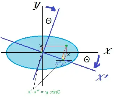
And so, we have an ellipsoidal, centered data cloud in the space of uncorrelated variables $X$ and $Y$. We have to rotate the axes by angle $\theta$. A data point in the cloud (such as shown as green spot on the picture) with $X$ coordinate $x$ will have this coordinate as $x^*$ after the rotation.

Observe that projection of the coordinate $x$ notch onto the rotated axis $X^*$ is given by $x'=x\cos\theta$ (cathetus as the hypotenuse and the angle between them). Observe also that $x^*$ is less than $x'$ by the cut of length $x'-x^*$ computable from coordinate $y$: $y\sin\theta$ (another cathetus and hypotenuse). And so,

$$x^* = x' - (x'-x^*) = x\cos\theta-y\sin\theta$$

We know (see the beginning) the variances (or sums-of squares) of the two variables and the variance (sum-of squares) $\mu^2$ of $X^*$. Then it follows:

$$\mu^2=\sum x^{*2} = \sum(x\cos\theta-y\sin\theta)^2 = \sum(x^2\cos^2\theta+y^2\sin^2\theta-2xy\cos\theta\sin\theta) = \cos^2\theta\sum x^2 + \sin^2\theta\sum y^2 - \underbrace{ 2\cos\theta\sin\theta\sum xy}_{\text{=0 (X and Y are uncorrelated)}} = \cos^2\theta (\sigma^2_{max}) + \sin^2\theta (\sigma^2_{min})$$

From which you estimate $\cos\theta$, as @amoeba has shown, and perform the rotation.

Answer 3

If I interpret things correctly, you mean that the first principle component (eigenvalue) explains most of the variance in the data. This can happen when your compression method is linear. However, there might be non-linear dependencies in your feature space.

TL/DR: PCA is a linear method. Use Autoencoders (non-linear pca) for dimensionality reduction. If the machine learning part is supervised learning then simply monitor your loss function while adjusting the (hyper)parameters for the autoencoder. In this way you will end up with a far better compressed version of your original data.

Here's a scikit example where they do grid search to find the optimal number of principal components to keep (hyper-parameter) using PCA. Finally they apply Logistic Regression on the lower dimensional space: http://scikit-learn.org/stable/auto_examples/plot_digits_pipe.html#example-plot-digits-pipe-py

Protip: Autoencoders do not have a closed form solution (afaik) so if your context is streaming data, this means you can continuously update your autoencoder (compressed representation) and can thus compensate for things such as concept drift. With pca you have to re-train batch mode from time to time as new data comes in.

As to giving some features more "weight", see regularization ( I'd start from norms https://en.wikipedia.org/wiki/Norm_(mathematics) ). You might also be surprised how similar logistic regression is to the perceptron.