4

Suppose $S$ is distributed as a Wishart matrix with $n$ degrees of freedom and scale matrix $\Sigma$, and let $\vec{a}$ be a fixed vector. It is well known that $\vec{a}^{\top}S\vec{a}$ is equal to $\vec{a}^{\top}\Sigma\vec{a}$ times a Chi-square random variable with $n$ degrees of freedom.

I am curious about the distribution of $\vec{a}^{\top}S^{-1}\vec{a}$. My guess was that it would be disributed as an inverse gamma, with scale $\vec{a}^{\top}\Sigma^{-1}\vec{a} / 2$, and shape $n/2$. My simulations (which are somewhat questionable) indicate this is not the case. Does this follow a well-known distribution?

shabbychef
  • 10,388
  • 7
  • 50
  • 93
  • 1
    You might be interested in [Chapter 8](http://projecteuclid.org/euclid.lnms/1196285114) from M. L. Eaton (2007), *Multivariate statistics: A vector-space approach*, Inst. Math. Stat. Lecture Notes, Monograph series. See, in particular, Proposition 8.9 on pages 312ff. – cardinal Oct 23 '11 at 21:51

2 Answers2

2

It does have an inverse gamma distribution, but not that one: it is actually an inverse gamma with parameters $\vec{a}^\top \Sigma^{-1} \vec{a} /2$ and $(n-p+1)/2$, where $p$ is the dimension of $S$.

The confusion is due to the marginal distribution of submatrices of the inverse Wishart. For example, if you choose $\vec{a} = (1,0,\ldots,0)^\top$, then: $$ \vec{a}^\top S^{-1} \vec{a} = [S^{-1}]_{11} $$ using the parameterisation of the Wikipedia page, this has a $W^{-1}\big( [\Sigma^{-1}]_{11},n-(p-1) \big)$ distribution.

Note that some papers, such as this one, use a different parameterisation of the inverse Wishart, such that if $U \sim IW(\delta; \Phi)$, then $U_{11} \sim IW(\delta; \Phi_{11})$, so you should check which one an author is using.

Simon Byrne
  • 3,336
  • 15
  • 29
1

Here is the simulation confirming @Simon Byrne's answer:

#demonstrate a'S a is inverse gamma when S is inverse Wishart W^-1(n,Sg^-1),
#for vector a, with scale a'Sg^-1 a / 2...
rwish <- function(n,Sg) {
  #generate variates from W(n,Sg) wishart distribution, the slow way
  #rwishart from bayesm library is probably faster
  C <- chol(Sg)
  p <- dim(Sg)[1]
  X <- matrix(rnorm(n*p),nrow=n) %*% C
  Z <- t(X) %*% X
}
rinvwishprod <- function(n,a,Sg=diag(x=1,nrow=length(a),ncol=length(a))) {
  #a' X a, where X is inv-wishart with parameters n and Sg^-1
  X <- rwish(n,Sg)
  t(a) %*% solve(X,a)
}
set.seed(1729)
n <- 256
p <- 16
ntrial <- 2048
#generate a PSD matrix Sg
X <- matrix(rnorm(2*p*p),nrow=2*p,ncol=p)
Sg <- t(X) %*% X
#generate vector a
a <- matrix(rnorm(p),nrow=p)
#draw many variates from this process
many.rv <- replicate(ntrial,rinvwishprod(n,a,Sg))
#try to transform to uniform RV using the inverse gamma law
alpha <- (n - p + 1) / 2
beta <- (t(a) %*% solve(Sg,a)) / 2
is.it.uniform <- pgamma(1 / many.rv,shape=alpha,rate=beta)
#plot the results
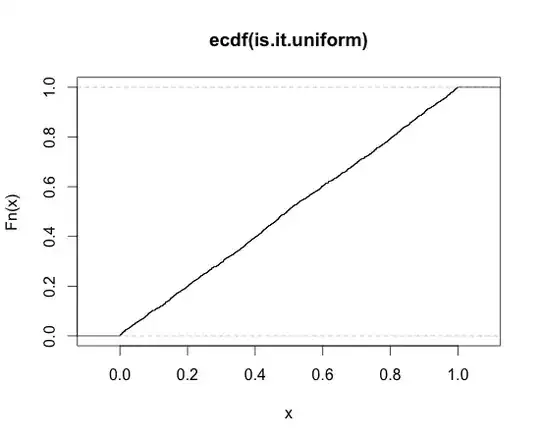
plot(ecdf(is.it.uniform))

Basically I generate, for fixed $\Sigma, n, \vec{a}$, variates of the form $v = \vec{a}^{\top}S^{-1}\vec{a}$, where $S \sim \mbox{W}\left(n,\Sigma\right)$, then compute the CDF under the inverse gamma relationship (shape parameter $\alpha = (n - p + 1)/2$ and scale parameter $\beta = \vec{a}^{\top}\Sigma^{-1}\vec{a}/2$). The resultant 'p-value' should be uniform, which is confirmed visually: p-value under inverse wishart to inverse gamma

shabbychef
  • 10,388
  • 7
  • 50
  • 93