Means of groups A and B differ significantly. I want to classify values into A or B

Question

My data look like this.

The variable on the $x$ axis is height in inches. The variable on the $y$ axis is whether someone hovers when urinating at a public toilet. Each of the 103 points is a female university student.

According to a $t$-test, the mean height of hoverers is significantly higher than that of non-hoverers.

I would like to make an inference in the opposite direction; I would like to know whether taller women are more likely to hover.

1. Is it reasonable to suspect based on my $t$-test that the opposite inference would hold?
2. A logistic regression found no significantly increased odds of hovering corresponding to an increase in height. Is there a different test I should try for this opposite relationship?

Answer 1

(1) Almost. A better comparison would be to a test of medians (like a rank sum test) rather than means. The means are sensitive to outlying data and the t-test is sensitive to skewed data. Moreover, if the medians are different then we have evidence that the proportion of taller people who are hoverers exceeds the proportion of shorter people who are, which is relevant to the prediction question. Nevertheless, using a t-test like this as an initial screen to identify potentially significant variables is standard. Hosmer and Lemeshow write,

...the linear discriminant function [which looks like a t statistic] and the maximum likelihood estimate of the logistic regression coefficient are usually quite close when the independent variable is approximately normally distributed within each of the outcome groups. ... Thus, univariable analysis based on the t-test should be useful in determining whether the variable should be included in the model, since the p-value should be of the same order of magnitude as that of the Wald statistic, Score test, or likelihood ratio test from logistic regression.

(Applied Logistic Regression, Second Edition, p. 93.)

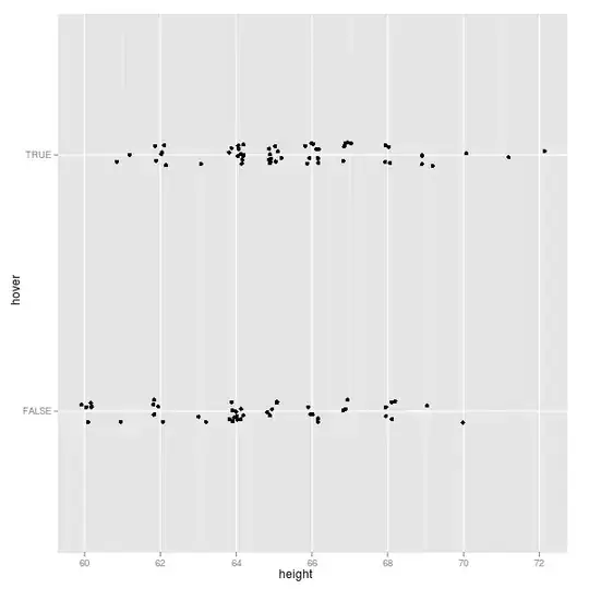
(2) It's hard to find 173 points in the plot; a close look identifies only 97 distinct markers. But let me use this to illustrate an approach.

Here are my data as counts:

Height Hovering Not hovering
60  0   5
61  2   1
62  6   5
63  1   2
64  11  11
65  10  4
66  9   5
67  5   3
68  4   5
69  3   1
70  1   1
71  1   0
72  1   0

A logistic regression has an overall p-value of .0616:

Logistic regression                               Number of obs   =         97
                                                  LR chi2(1)      =       3.49
                                                  Prob > chi2     =     0.0616
Log likelihood = -64.863893                       Pseudo R2       =     0.0262

------------------------------------------------------------------------------
      hovers |      Coef.   Std. Err.      z    P>|z|     [95% Conf. Interval]
-------------+----------------------------------------------------------------
      height |   .1539169   .0845634     1.82   0.069    -.0118243    .3196581
       _cons |   -9.76445   5.488694    -1.78   0.075    -20.52209    .9931935
------------------------------------------------------------------------------

Although this is not "significant" at any level more stringent than 6%, it's suggestive, and the coefficient of 15% per inch is large. One reason the regression can fail to be as significant as the t-test (or other tests) is that the relationship between the log odds and the height might be nonlinear. To evaluate this, bin the heights and compute the logits of the proportions (of hoverers to total subjects) within each bin. (Doing this is a good idea for checking the fit of any logistic regression, because the model assumes the logits will vary linearly with the independent variables.) To handle zero counts, I have added 1/6 to every count before performing the calculations.

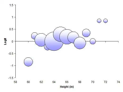
The areas of the plot symbols are proportional to the total counts in each (one-inch) height bin. There is a trend, but it is strongly s-shaped, not linear. It is most heavily influenced by the leftmost point (all women 60 inches tall), which has a fair weight (it represents about 5% of the subjects) and large leverage (because it is at an extreme value of the independent variable). I would discount the two small symbols at the upper right, because they represent just two individuals: there is a lot of uncertainty as to their correct positions. But let's not throw them away!

This plot ought to remind us of the biophysics of the problem. I'm not exactly sure what "hovering" is, but I suspect it's a physical activity that requires a minimum height for efficacy, or at least becomes disproportionately more difficult to do at less than the threshold height. People near or below that threshold will necessarily be in the non-hovering class, regardless of preference or any other mechanism relating hovering to height. The plot provides evidence that this threshold is between 60 and 61 inches. Accordingly, it would make sense to check for a separate trend only among all subjects 61 inches or taller. This time, the p-value of the logistic regression is 0.439, agreeing with the visual impression of practically no trend among all the dots. (It still has a positive coefficient, though, of about 7% per inch. This is substantial enough that we might be interested in prolonging the study to see whether the effect is really due to chance, as the p-value hints, or represents a real trend.)

Based on this version of the data (which may be incorrect), we would conclude that:

• There is some evidence of a threshold effect around 60-61 inches.

• Otherwise there is no evidence of any regular trend in hovering propensity with height.

Because I have used an exploratory analysis to suggest this model, it wouldn't be right to use the same data to confirm the model with formal hypothesis tests. But perhaps going into exploratory mode provides more insight, if less certainty, than routine (and blind) application of statistical tests.