This post is about 2800 words long in order to handle the response to comments. It looks much larger due to the size of the graphics. About half the post in length is graphics. Nonetheless, a comment makes mention that with my edit, the whole is difficult to consume. So what I am doing is providing an outline and a restructuring to make it easier to know what to expect.
The first section is a brief defense of the use of Frequentist methods. All too often in these discussions people bash one tool for another. The second is a description of a game where Bayesian method guarantee the user of Frequentist methods takes a loss. The third section explains why that happens.
A DEFENSE OF FREQUENTISM
Pearson and Neyman originated statistics are optimal methods. Fisher's method of maximum likelihood is an optimal method. Likewise, Bayesian methods are optimal methods. So, given that they are all optimal in at least some circumstances, why prefer non-Bayesian methods to Bayesian ones?
First, if the assumptions are met, the sampling distribution is a real thing. If the null is true, the assumptions hold, the model is the correct model and if you could do things such as infinite repetition, then the sampling distribution is exactly the real distribution that nature would create. It would be a direct one-to-one mapping of the model to nature. Of course, you may have to wait an infinite amount of time to see it.
Second, non-Bayesian methods are often required by statute or regulation. Some accounting standards only are sensible with a non-Bayesian method. Although there are workarounds in the Bayesian world for handling a sharp null hypothesis, the only type of inferential method that can properly handle a hypothesis such as $H_0:\theta=k$ with $H_A:\theta\ne{k}$ is a non-Bayesian method. Additionally, non-Bayesian methods can have highly desired properties that are unavailable to the Bayesian user.
Frequentist methods provide a guaranteed maximum level of false positives. Simplifying that statement, they give you a guarantee of how often you will look like a fool. They also permit you to control against false negatives.
Additionally, Frequentist methods, generally, minimize the maximum amount of risk that you are facing. If you lack a true prior distribution, that is a wonderful thing.
As well, if you need to do transformations of your data for some reason, the method of maximum likelihood has wonderful invariance properties that usually are absent from a Bayesian method.
Problematically, Bayesian calculations are always person-specific. If I have a highly bigotted prior distribution, it can be the case that the data collected is too small to move it regardless of the true value. Frequentist methods work equally well, regardless of where the parameter sits. Bayesian calculations do not work equally well over the parameter space. They are best when the prior is a good prior and worst when the prior is far away.
Finally, Bayesian reasoning is always incomplete. It is inductive. For example, models built before relativity would always be wrong about things that relatively impacts. A Frequentist test of Newtonian models would have rejected the null in the edge cases such as the orbit of Mercury. That is complete reasoning. Newton is at least sometimes wrong. It is true you still lack a good model, but you know the old one is bad. Bayesian methods would rank models and the best model would be a bad model. Its reasoning is incomplete and one cannot know how it is wrong.
Now let us talk about when Bayesian methods are better than Frequentist methods. There are three places where that happens, except when it is required by some rule such as an accounting standard.
The first is when you are needing to update your beliefs or your organization's beliefs. Bayesian methods separate Bayesian inference from Bayesian actions. You can infer something and also do nothing about it. Sometimes we do not need to share an understanding of the world by agreeing on accepting a convention like a t-test. Sometimes I need to update what I think is happening.
The second is when real prior information exists but not in a form that would allow something like a meta-analysis. For example, people investing in riskier assets than bonds should anticipate receiving a higher rate of return than bonds. If you know the nominal interest rate on a bond of long enough duration, then you should anticipate that actors in the market are attempting to earn more. Your prior should reflect that is improbable that the center of location for stocks should be less than the return on bonds. Conversely, it is very probable that is greater, but not monumentally greater either. It would be surprising for a firm to be discounted in a competitive market to a 200% per year return.
The third reason is gambling. That is sort of my area of expertise. My area can be thought of as being one of two things. The first is the study of the price people require to defer consumption. The second would be the return required to cover a risk.
In the first version, buying a two-year-old a birthday present in order to see them smile next week is an example of that. It is a gamble. They may fall in love with the box and ignore the toy breaking our hearts and making them happy. In the second, we consider not only the raw outcome but the price of risk. In a competition to own or rid oneself of risk, prices form.
In a competitive circumstance, the second case and not the first, only Bayesian methods will work because non-Bayesian methods and some Bayesian methods are incoherent. A set of probabilities are incoherent if I can force a middleman such as a market maker or bookie to take a loss.
All Frequentist methods, at least some of the time, when used with a gamble can cause a bookie or market maker to take a loss. In some cases, the loss is total. The bookie will lose at every point in the sample space.
I have a set of a half-dozen exercises that I do for this and I will use one below. Even though the field of applied finance is Frequentist, it should not be. See the third section for the reason.
THE EXAMPLE
As you are a graduate statistics student, I will drop the story I usually tell around the example so that you can just do the math. In fact, this one is very simple. You can readily do this yourself.
Choose a rectangle in the first quadrant of a Cartesian plane such that no part of the rectangle touches either axis. For the purposes of making the problem computationally tractable, give yourself at least some distance from both axes and do not make it insanely large. You can create significant digit issues for yourself.
I usually use a rectangle where neither $x$ nor $y$ is less than 10 and nothing is greater than 100, although that choice is arbitrary.
Uniformly draw a single coordinate pair from that plane. All the actors know where the rectangle is at so you have a proper prior distribution with no surprises. This condition exists partly to ground the prior, but also because there exist cases where improper priors give rise to incoherent prices. As the point is only to show differences exist and not to go extensively into prior distributions, a simple grounding is used.
The region doesn't have to be a rectangle. If you hate yourself, make a region shaped like an outline of the Statue of Liberty. Choose a bizarre distribution over it if you feel like it. It might be unfair to Frequentist methods to choose a shape that is relatively narrow, particularly one with something like a donut hole in it.
On that rectangle will be placed a unit circle. There is nothing special about a circle, but unless you hate yourself, make it a circle that is small relative to the rectangle. If you make it too small, again, you could end up with significant digit issues.
You will be the bookie and I will be the player. You will use Frequentist methods and I will use Bayesian methods. I will pay an upfront lump sum fee to you to play the game. The reason is that a lump sum is a constant and will fall out of any calculations about profit maximization. Again, if you hate yourself, do something else.
You agree to accept any finite bet that I make, either short or long, at your stated prices. You also agree to use the risk-neutral measure. In other words, you will state fair Frequentist odds. Your sole source of profit is your fee, in expectation. We can assume that you have nearly limitless pocket depth compared to my meager purse.
The purpose of this illustration is to illustrate an example of how a violation of the converse of the Dutch Book Theorem, or the Dutch Book Theorem, assures bad outcomes. You can arbitrage any Frequentist pricing game, though not necessarily in this manner.
The unit circle is in a position unknown to either of us. The unit circle will emit forty points drawn uniformly over the circle. You will draw a line from the origin at $(0,0)$ through the minimum variance unbiased estimator of the center of the circle. The line is infinitely long so you will cut the disk into two pieces.
We will gamble whether the left side or the right side is bigger. Because the MVUE is guaranteed to be perfectly accurate by force of math, you will offer one-to-one odds for either the left side or the right side. How will I win?
As an aside, it doesn't matter if you convert this to polar coordinates or run a regression forcing the intercept through the origin. The same outcome ends up happening.
So first understand what a good and bad cut would look like.
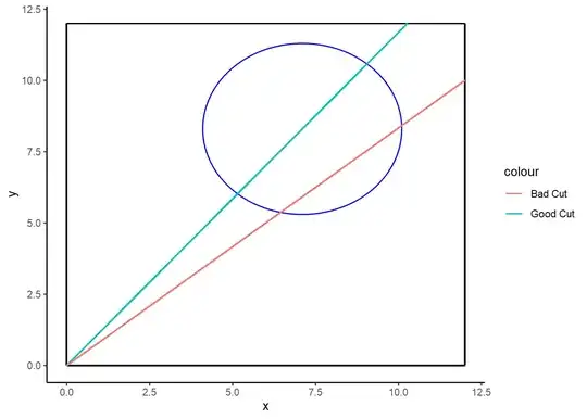
In this case, the good cut is perfect. Every other cut is in some sense bad.
Of course, neither you nor I get to see the outline. We only get to see the points. 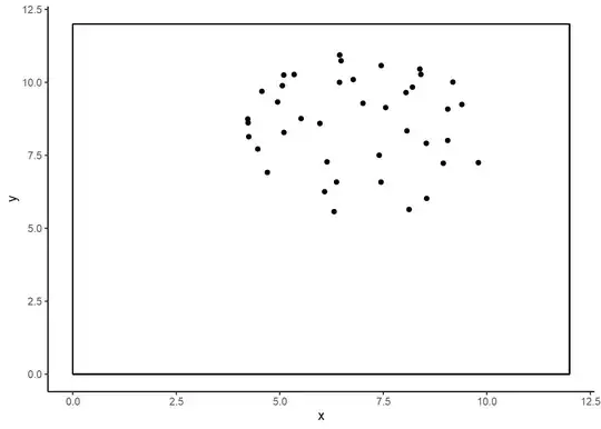
The Frequentist line passes through the MVUE. Since the distribution of errors are symmetric over the sample space, one-to-one odds should not make you nervous. 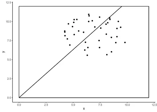
It should make you nervous, though. All of the information about the location of the disk comes from the data alone with the Frequentist method. That implies that the Bayesian has access to at least a trivial amount of extra information. So I should win at least on those rare happenings where the circle is very near to the edge and most of the points are outside the rectangle. So I have at least a very small advantage, though you can mitigate it by making the rectangle comparatively large.
That isn't the big issue here. To understand the big issue, draw a unit circle around the MVUE. 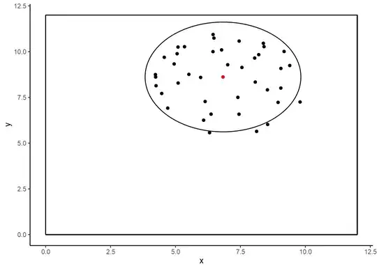
You now know, for sure, that the left, upper side is smaller than the opposite with perfect certainty. You can know this because some points are outside the implied circle. If I the Bayesian can take advantage of that, then I can win anytime the MVUE sits in an impossible place. Any Frequentist statistic can do that. Most commonly, it happens when the left side of a confidence interval sits in an impossible location as may happen when it is negative for values that can only be positive.
The Bayesian posterior is always within one unit of every single point in the data set. It is the grand intersection of all the putative possible circles drawn around every point. The green line is the approximation of the posterior, though I think the width of the green line might be a bit distorting. The black dot is the posterior mean and the red dot the MVUE.
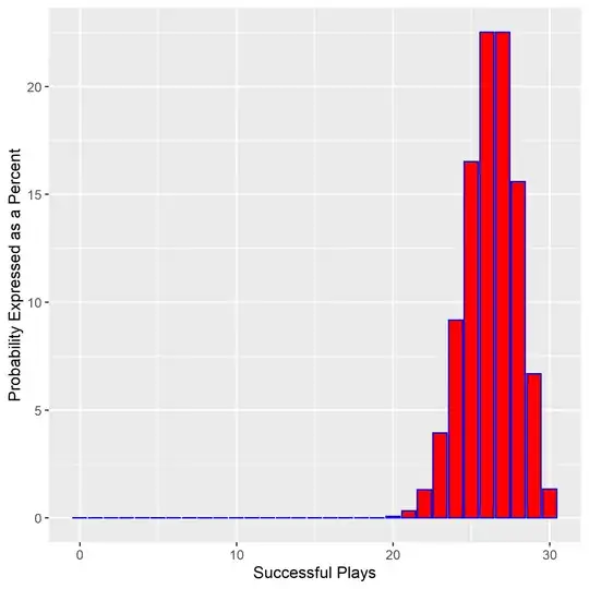
The black circle is the Bayesian circle and the red circle the Frequentist one. In the iteration of this game that was used to make this example, I was guaranteed a win 48% of the time and won roughly 75% of the remaining time from the improved precision. If you make Kelly Bets for thirty rounds, you make about 128,000 times your initial pot.
Under Frequentist math, you expected to see this distribution of wins over thirty rounds.
The Bayesian player expects to win under this distribution.
Technical Aside
It is not sufficient for the MVUE to be outside the posterior. It must also be outside the marginal posterior distribution of the slope. There do exist circumstances where the Frequentist line is possible even though the Frequentist point is not. Imagine the Bayesian posterior as a cone from the origin. The MVUE can be outside the posterior but inside the cone. In that circumstance, you bet the Kelly Bet based on the better precision of the Bayesian method. Also, improper priors can also lead to incoherence.
Note On Images
The boxes in the images were to make the overall graphic look nice. It wasn't the boundary I actually used.
WHY THIS HAPPENS
I have a half-dozen of these examples related to market trading rules. Games like this are not that difficult to create once you notice that they exist. A cornucopia of real-world examples exists in finance. I would also like to thank you for asking the question because I have never been able to use the word cornucopia in a sentence before.
A commentator felt that the difference was due to allowing a higher level of information by removing the restriction on an estimator being unbiased. That is not the reason. I have a similar game that uses the maximum likelihood estimator and it generates the same type of result. I also have a game where the Bayesian estimator is a higher variance unbiased estimator and it also leads to guaranteed wins. The minimum variance unbiased estimator is precisely what it says it is. That does not also imply that it is coherent.
Non-Bayesian statistics, and some Bayesian statistics, are incoherent. If you place a gamble on them, then perfect arbitrage can be created at least some of the time. The reason is a bit obscure, unfortunately, and goes to foundations. The base issue has to do with the partitioning of sets in probability theory. Under Kolmogorov’s third axiom, where $E_i$ is an event in a countable sequence of disjoint sets $$\Pr\left(\cup_{i=1}^\infty{E_i}\right)=\sum_{i=1}^\infty\Pr(E_i),$$ we have at least a potential conflict with the Dutch Book Theorem. The third result of the Dutch Book Theorem is $$\Pr\left(\cup_{i=1}^N{E_i}\right)=\sum_{i=1}^N\Pr(E_i),N\in\mathbb{N}.$$ It turns out that there is a conflict.
If you need to gamble, then you need sets that are finitely but not countably additive. Furthermore, in most cases, you also need to use proper prior distributions.
Any Frequentist pricing where there is a knowledgeable competitor leads to arbitrage positions. It can take quite a while to figure out where it is at, but with effort it can be found. That includes asset allocation models when when $P=P(Q)$. Getting $Q$ wrong shifts the supply or demand curves and so gets $P$ wrong.
There is absolutely nothing wrong with the unbiased estimators in the example above. Unbiased estimators do throw away information, but they do so in a principled and intelligently designed manner. The fact that they produce impossible results in this example is a side-effect anyone using them should be indifferent to. They are designed so that all information comes from the data alone. That is the goal. It is unfair to compare them to a Bayesian estimator if your goal is to have all information come from the data. The goal here isn’t scientific; it is gambling. It is only about putting money at risk.
The estimator is only bad in the scientific sense because we have access to information from outside the data that the method cannot use. What if we were wrong and the Earth was round, angels do not push planets around and spirits do not come to us in our dreams? Sometimes not using outside knowledge protects science. In gambling, that is a bad idea. A horse that is a bad mudder is important information to include if it just rained, even if that is not in your data set.
This example is primarily to show that it can be done and produces uniquely differing results. Real prices often sit outside the dense region of the Bayesian estimation. Warren Buffet and Charlie Munger have been able to tell you that since before I was born, as was Graham and Dodd before them. They just were not approaching it in the framework of formal probability. I am.
It is the interpretation of probability that is the problem, not the bias or lack thereof. Always choose your method for fitness of purpose, not popularity. Our job is to do a good job, not be fashionable.


