Why are coefficients estimates more accurate when using a hierarchical model?

Question

I am reading a paper and I do not understand a bit: "We use a hierarchical model such that all slopes are calculated within the same model and the intercepts and slope components are normally distributed among columns. This results in more accurate coefficient estimates."

I would like to understand why do we expect coefficient estimates to be more accurate.

Is it because less information is discarded as there is a use of mean and variance and a normal distribution can be described using only those?

Can you share more, or perhaps a paper link or citation? (I suspect you'll get a better answer if more specifics are known.) — Sean Easter, Aug 05 '15 at 01:50
I think it is related to the Philosophy of hierarchical model, because it can deal non i.i.d to some extent. — Deep North, Aug 05 '15 at 01:53
The paper is unpublished and I am not allowed to share it, unfortunately. — Julian Wittische, Aug 08 '15 at 20:39

score 2 · Accepted Answer · answered Aug 14 '15 at 23:04

The coefficient estimates are said to be more accurate because the hierarchical model has less model variance than the alternative (which I'll assume is a linear model). It achieves this by pooling the information across predictors into overall estiamtes.

Here is an extreme example with random intercepts. Suppose I generate some data with a categorical predictor with a large number of levels, but so that the predictor has absolutely no relationship to the response:

N <- 5000
N.classes <- 500

rand.class <- factor(sample(1:N.classes, N, replace=TRUE))
y <- rnorm(N)

Estimating a linear model from this data yields highly inaccurate coefficient estimates

lin.mod <- lm(y ~ rand.class)

plot(seq_along(lin.mod$coefficients), lin.mod$coefficients, 
               main="Estimated Coefficients: Linear Model",
               xlab="Coefficient Id",
               ylab="Estimate")

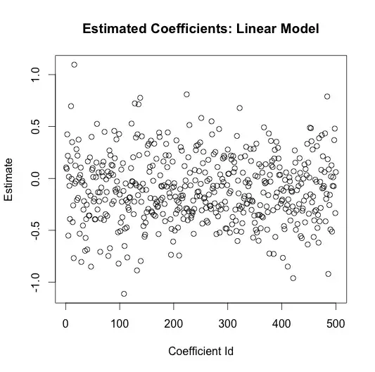
The average coefficient estimate is

> mean(lin.mod$coefficients)
[1] 0.1686486

and their standard deviation is

> sd(lin.mod$coefficients)
[1] 0.3524578

The true value for every one of these coefficients is zero. The linear model did not figure this out, it gleefully attributed random variation in the data to signal.

Now let's fit a random intercept model from exactly the same data.

library(lme4)
library(arm)
lme.mod <- lmer(y ~ (1 | factor(rand.class)) - 1)

Here a summary of the model's findings

> display(lme.mod)
lmer(formula = y ~ (1 | factor(rand.class)) - 1)
coef.est  coef.se 
    0.00     0.01 

Error terms:
 Groups             Name        Std.Dev.
 factor(rand.class) (Intercept) 0.00    
 Residual                       0.99    
 ---
 number of obs: 5000, groups: factor(rand.class), 500

The average coefficient (0.00) and their standard deviation (0.01) are much more accurately estimated. The model also attributes almost all of the variance to noise (0.99), which is quite close to the truth (its all noise).

A scatter of the coefficients shows the dramatic difference

lme.coefficients <- ranef(lme.mod)$rand.class[,1]
plot(seq_along(lme.coefficients), lme.coefficients, 
     main="Estimated Coefficients: Random Intercepts Model",
     xlab="Coefficient Id",
     ylab="Estimate",
     ylim=c(-1.1, 1.1))

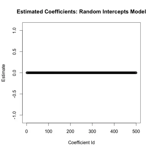
I purposefully plotted these on the same scale as the coefficients from the linear model to highlight the dramatic reduction in variance. All the coefficients are estimated to be essentially zero, which is the truth.

What happen here is something like the following. The linear model assumes no relationship between the coefficient estimates for the individual factors, each is estimated independent of the others, and is completely unconstrained to live anywhere along the number line; this results in the coefficients being highly sensitive to the training data. On the other hand, the random intercept model attempts to enforce a distribution to the coefficient estimates

$$ \alpha \sim N(\mu, \sigma) $$

This ties the coefficient estimates together holistically, and allows information to be "pooled" across the estimates, reducing the sensitivity to training data.

Why are coefficients estimates more accurate when using a hierarchical model?

1 Answers1

Linked