6

I need to identify seasonality/ periodicity of a dataset so as to develop an ARMAX model. This is what the original time-series looks like enter image description here

I have plotted the periodogram of the dataset.

Ps: I used the first difference of the original time series so as to remove the trend from the original time series . This what the periodogram looks likeenter image description here
I also removed the linear trend from the data and estimated the periodogram. Below is what it looks like

enter image description here

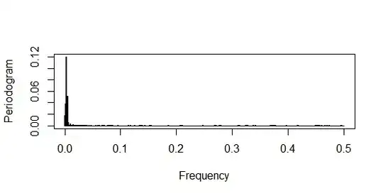
I also estimated periodogram of the raw data set without any differencing. Clearly, it shows there is some trend in the data. I am using following R-code to generate it

A <- read.xlsx("Interpolation_Data.xlsx")
y <- A[,2]
x <- as.numeric(A[,4])
diff.y <- diff(y)
diff.x <- diff(x)
Fs<- 1/60
n=length(diff.y)
xdft <-fft(diff.y)
xdft <- xdft[1:(n/2+1)]
psdx <- (1/(Fs*n))* abs(xdft)^2
psdx[c(-1,-n)] <- 2*psdx[c(-1,-n)]
f <- seq(0,Fs/2,by = Fs/n)
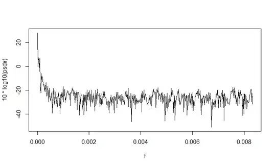
plot(f,10*log10(psdx),type='l')
This is the link to data set

Spandyie
  • 393
  • 4
  • 13

1 Answers1

6

Well, the periodogram after taking first differences doesn't indicate any clear periodicity. However, be aware that taking first differences amplifies high-frequency components, which should appear in the power spectrum as a quadratic trend, and in the log-power spectrum as a log-shaped trend (which is roughly compatible with what we see here).

My recommendations:

– First compute the periodogram without any preprocessing.

– Then, remove the linear trend, but not by using first differences but by fitting a line by regression and subtracting the result from the data (there should also be a "detrend" function in R).

– Use a proper spectral estimation function. I'm not familiar with R, but I'm sure it contains an implementation of Welch's modified periodogram method.


Update for the updated question:

The time series exhibits a dominant period of roughly 360 samples, which for a sampling rate of 1 per minute means 360 minutes. The dominant frequency should therefore be about 0.0028 min$^{-1}$. This seems to be consistent with the periodogram after subtracted trend. Try zooming into the low-frequency range to more precisely determine the peak location. Superimposed to that is a secondary oscillation of 180 samples period or 0.0056 min$^{-1}$ frequency.

Analyzing your data myself I get a main peak at 0.0029 min$^{-1}$ and a secondary peak at 0.0059 min$^{-1}$ (factor 2, the first harmonic). The secondary peak is smaller by a factor of about 36, or by 16 dB. I can share my code, but I am using Matlab, not R.

Btw., the frequency scale on your plots does not appear to be consistent; sometimes it goes up to 0.008, sometimes to 0.5? I think the former gives the frequency in Hz and the latter in min$^{-1}$.

A. Donda
  • 2,819
  • 14
  • 32
  • I have also attached the periodogram on a raw time series data without any preprocessing. – Spandyie Jul 22 '15 at 16:33
  • 1
    @Spandy, thanks, but now I feel that this spectrum might actually be disturbed by a trend (the strong increase towards 0 is an indicator). Would you also follow my second recommendation: subtract a linear trend? – A. Donda Jul 22 '15 at 19:09
  • I have included the original time series data in the new edit. Also I detrended the data and estimated the periodogram as you suggested. The results have slightly improved, but the lower frequency components are still dominant. Any comments you have ? – Spandyie Jul 22 '15 at 20:52
  • 1
    @Spandy, see my updated answer. – A. Donda Jul 23 '15 at 02:10
  • I am getting dominant frequency to be 0.003125, not precisely equals to what you are getting but some what close. Also, in the detrended periodogram I am using normalized frequency. Do you mind sharing your Matlab code, may be I can use that to compare against my code? Thanks in advance . – Spandyie Jul 23 '15 at 02:50
  • 1
    @Spandy, in this case normalized frequency is identical to frequency in min$^{-1}$, because the sampling rate is 1 (per minute). I think in this case that's the most useful frequency scale. – The difference in estimated peak frequency is probably due to the fact that the algorithm I use 0-padded the time series to 1024 samples before spectral analysis; with such a slow rhythm it is hard to determine the frequency exactly. – A. Donda Jul 23 '15 at 02:58
  • 1
    My code: `x = detrend(x); [P, fs] = pwelch(x, numel(x), [], [], 1); semilogy(fs, P, '.-')`, using `pwelch` from Matlab's *Signal Processing Toolbox*. – If my answer helped you, consider accepting it. – A. Donda Jul 23 '15 at 02:59
  • 1
    really appreciate your help – Spandyie Jul 23 '15 at 03:04