Yes, the approaches give the same results for a zero-mean Normal distribution.
It suffices to check that probabilities agree on intervals, because these generate the sigma algebra of all (Lebesgue) measurable sets. Let $\Phi$ be the standard Normal density: $\Phi((a,b])$ gives the probability that a standard Normal variate lies in the interval $(a,b]$. Then, for $0 \le a \le b$, the truncated probability is
$$\Phi_{\text{truncated}}((a,b]) = \Phi((a,b]) / \Phi([0, \infty]) = 2\Phi((a,b])$$
(because $\Phi([0, \infty]) = 1/2$) and the folded probability is
$$\Phi_{\text{folded}}((a,b]) = \Phi((a,b]) + \Phi([-b,-a)) = 2\Phi((a,b])$$
due to the symmetry of $\Phi$ about $0$.
This analysis holds for any distribution that is symmetric about $0$ and has zero probability of being $0$. If the mean is nonzero, however, the distribution is not symmetric and the two approaches do not give the same result, as the same calculations show.
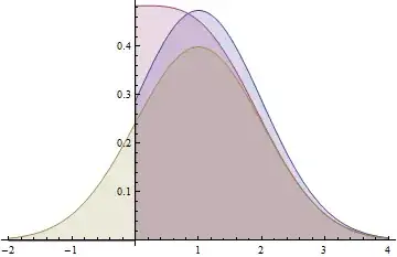
This graph shows the probability density functions for a Normal(1,1) distribution (yellow), a folded Normal(1,1) distribution (red), and a truncated Normal(1,1) distribution (blue). Note how the folded distribution does not share the characteristic bell-curve shape with the other two. The blue curve (truncated distribution) is the positive part of the yellow curve, scaled up to have unit area, whereas the red curve (folded distribution) is the sum of the positive part of the yellow curve and its negative tail (as reflected around the y-axis).
