I assume that you are trying to split the time series in the form:
y(t) = Trend(t) + Seasonality(t) + Random(t), given the measurements are taken after equal time intervals.
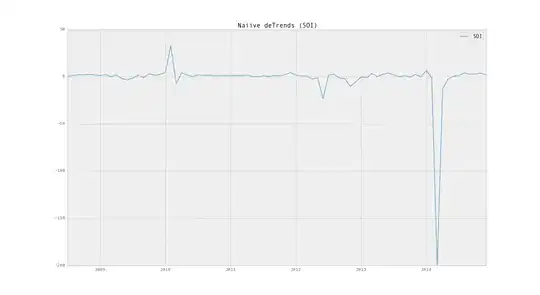
In general, the trend is a polynomial function of time. Therefore continuous differencing will detrend the series (but will create a completely different series). Eg: If the original series is I(1), then let z(t) = y(t+1) - y(t) for t = 1, 2, ..., n-1. If y has a linear trend, then z will be trendless. However, if y has higher order trend, then define p(t) = z(t+1) - z(t), q(t) = p(t+1) - p(t), ... till the final series becomes trendless. This process should be stopped when the first trendless series is obtained.
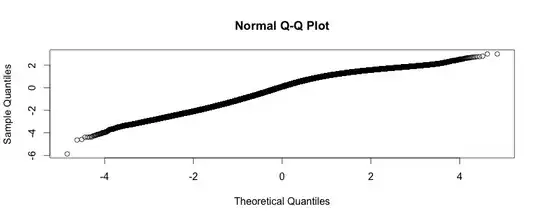
Presence of trend can be verified using Augmented Dickey-Fuller test. Use the following command in R: adf.test(column_vector) -> replace column_vector with z, p or q respectively.
Alternative:
You can use the command decompose in R. Given the seasonality, it will automatically split the time series into trend, seasonal and random components.
Caution:
Don't use log transformation unless the log(y2) - log(y1) makes sense. For example, in case of daily stock price data, log(y2) - log(y1) = Return on stock for 1 day.
Multiplicative Time Series:
Please refer this link
Another method:
You would be having the timestamps (t) associated with each observation. Remove the seasonal component and obtain another series x(t) = y(t) - Seasonality(t). Now regress x(t) with t and check for significance of coefficient of t. If it is significant with p-value < alpha, trend is a polynomial of order (at least) 1. Now add another column (t2) that is equal to square of the timestamp. Regress x(t) with t and t2 and check for significance of coefficient of t2. If it is significant, trend is a polynomial of order (at least) 2. Otherwise the trend is a polynomial of order = 1. Now add column t3, t4, ... till the order of the polynomial can be ascertained.
You can subtract beta1*t + beta2*t2 + ... + betan*tn from y(t) to detrend the series.