Simulate from a dynamic mixture of distributions, honoring the tail

Question

This question is a follow-up to this other question, brilliantly answered by Xi'an.

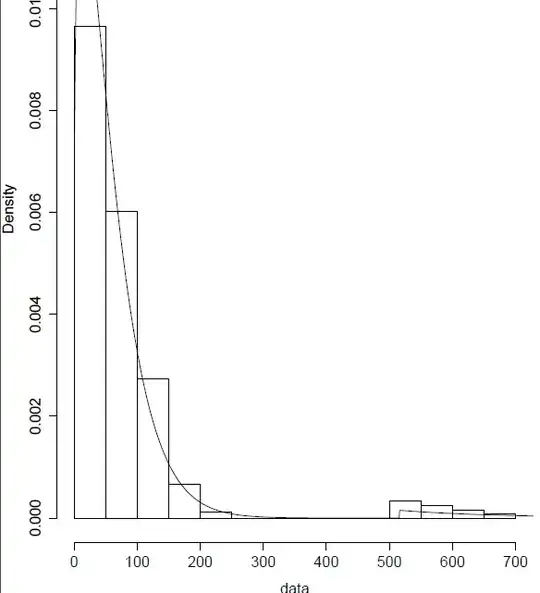
I have a dynamic mixture of Weibull and GPD distributions (with a CDF Cauchy mixing function). The mixture is fitted (I have all parameters), and looks like:

# this is reproducible R code    
libs=c("repmis","fExtremes","evmix","evir")
lapply(libs,library,character.only=TRUE)

cc=1.05
mixture=function(x){(1/cc)*((1-pcauchy(x, location=5.160288e+02,scale=8.364144e-04))*dweibull(x, shape=1.212213e+00,scale=5.877943e+01)+pcauchy(x, location=5.160288e+02,scale=8.364144e-04)*dgpd(x, xi=8.952331e-02, mu=0, beta=1.206929e+02))[1]}

data=source_data("https://www.dropbox.com/s/r7i0ctl1czy481d/test.csv?dl=0")[,1]
xeval=seq(min(data),max(data)+sd(data),length=length(data))

distr=numeric(length=length(xeval))
for(i in 1:(length(xeval))){
distr[i]=(mixture(xeval[i]))
}

hist(data,prob=TRUE,ylim=range(distr))
lines(xeval,distr,type="l")

I am trying to implement the following accept-reject simulation scheme (from Figressi et al. 2002, page 6):

1. draw $u$ uniformly on $[0,1]$
2. if $u<0.5$, sample $x$ from the Weibull distribution. Record $x$ with probability $1-p(x)$, or go back to step 1 with probability $p(x)$
3. if $u>=0.5$, sample $x$ from the GPD distribution. Record $x$ with probability $p(x)$, or go back to step 1 with probability $1-p(x)$

$p(x)$ is the CDF of the Cauchy distribution evaluated in $x$: $1/2 +(1/\pi)*arctan[(x-m)/\tau]$ (refer to the abovelinked question for more context).

This is what I have written in R:

nsim=1e4
simulation=numeric(length=nsim)

for (i in 1:nsim){

# step 1
u=runif(1)

# step 2
if (u<0.5){ 
# sample from Weibull
sample=(1/cc)*rweibull(n=1,shape=1.212213e+00,scale=5.877943e+01)

prob=(1-pcauchy(sample,location=5.160288e+02,scale=8.364144e-04))

if(runif(1)<prob){
  # accept
  simulation[i]=sample 
} else {
  # reject (cannot "go back" to step 1 so just allocate a value that will be removed later on)
  simulation[i]=-999
}
} else { # (step 3) 

# sample from GPD
sample=(1/cc)*rgpd(n=1,xi=8.952331e-02,mu=0,beta=1.206929e+02)

prob=pcauchy(sample,location=5.160288e+02,scale=8.364144e-04)

if(runif(1)<prob){
  # accept
  simulation[i]=sample 
} else {
  # reject
  simulation[i]=-999
}

}
}

# remove the "go back to step 1" values
simulation=simulation[simulation[]!=-999]

Plotting the results, it seems at first that the simulated values reproduce the little bump in the tail:

 hist(data,prob=T,ylim=range(density(simulation)$y));lines(density(simulation)$x,density(simulation)$y,lty=2)

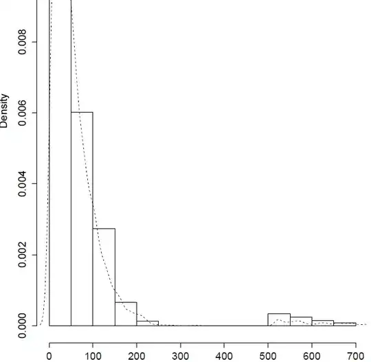
But actually, the tail is not well captured:

> quantile(simulation,0.97)
     97% 
208.5264 
> quantile(data,0.97)
     97% 
547.9452

The point of simulating here is to generate unseen extremes to faithfully account for risk, but the risk turns out to be severely underestimated... Is there a problem in my code? Any thoughts on how to honor the tail better?