Common trends with Difference in differences

Question

For OLS to have good properties, we should assume that $E(u|X)=0$. When using DiD, is it then this assumption which requires the so-called common trend assumption (need for the DiD to have good properties). If not, where then does the common trends assumption orignites from?

Answer 1

The fundamental problem with causal inference is that we never observe what would have happened to the treated if the treatment had not occured. If I give you a million dollars now, and next month I compare your consumption to what it is today then I will perhaps not get the treatment effect. Why? Perhaps your consumption next month would have changed anyway even if I had not given you all that money, for instance because the weather gets better and next month you buy some ice cream more. In that case we over-state the treatment effect.

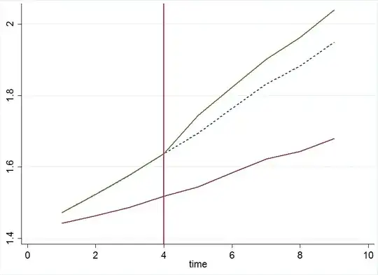
Consider the following graph and let's say you are treated and I'm control. The green line shows the evolution of your observed consumption over time for the treatment group and the same is shown for the control group with the red line. In period 4 you get a million dollars and from there our consumption diverges. The "treatment effect" is then the difference between the green line and the dashed blue line. The dashed blue line is our "counterfactual". It shows how your consumption would have developed if you had not gotten the million dollars - maybe. Of course we never observe the blue dashed line. But because you and I had the same trend in our consumption it is reasonable to assume that this is what would have happened.

This is probably the main point which does not come out as clearly as in the graph of the answer I had linked in the comment.

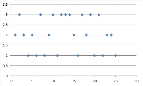
You probably understood the importance of the common trend assumption but let's give the counter-example. If you and I don't share a common trend in consumption, then DiD makes a pre- and post-treatment comparison between two groups that were not comparable with each other even before the treatment. See the graph below.

Now we don't have a counterfactual anymore because we cannot assume that your blue dashed line (which we don't observe) would behave the same way after the treatment as my observed red line. Now one might be tempted to say: "So I use my own pre-treatment trend to extrapolate". In this graph it seemingly works because everything is nice and pretty much linear but of course that's not how it works in reality. You can not know because it's a counterfactual! Also before we could not know with certainty but at least we could compare you and me and get a bit of an idea of how your counterfactual would like like. You also see that the "treatment effect" increases over time and you will realize that this is probably not because of the treatment.

To wrap up, let's throw in some maths as well:
Let $A$ be the post period (after), and $B$ the pre-treatment period (before), $Y^0$ is the potential(!) outcome and $D$ is a dummy which equals one if treated and zero otherwise. The bias of DiD is $$\text{bias}_{DID} = E\left[Y^0_A - Y^0_B|D = 1\right] - E\left[Y^0_A - Y^0_B|D = 0\right]$$

This just says that the bias of DiD is the change over time in the difference in potential outcomes for the treatment group versus the control group in the absence of the treatment (the difference between the red and the dashed blue line). This means that assuming parallel trends means to assume zero bias - that's why it is an important assumption and why it is important to show parallel trends if you want to convince your audience. You can find the formula for the bias in Chabé-Ferret (2014).