I have some data that tracks 2 variables over time. Let's call them A and B. So I have data on A and B for 15 years. I know how to calculate the correlation coefficient, but my goal is to see if the correlation between the two is increasing over time. If anyone knows of a way to do this I would really a precise your input!
Asked
Active
Viewed 2,956 times
2
kjetil b halvorsen
- 63,378
- 26
- 142
- 467
Kelly
- 21
- 1
- 3
-
1So, what is the problem? Calculate correlation across the whole time frame (saving in some structure both correlation coefficient and date/time stamp), which essentially will produce a time series. Then plot it and/or analyze analytically, depending on your needs. – Aleksandr Blekh Apr 08 '15 at 18:01
-
You could estimate & plot a conditional correlation, see https://stats.stackexchange.com/questions/235442/investigate-correlation-conditional-on-a-threshold/299958#299958 and https://stats.stackexchange.com/questions/203494/can-i-analyze-or-model-a-conditional-correlation/368228#368228, https://stats.stackexchange.com/questions/239645/what-is-the-physical-significance-of-cumulative-correlation-coefficient/371412#371412 – kjetil b halvorsen Aug 13 '19 at 07:32
3 Answers
3
You can estimate a time-varying coefficient in a linear regression model. To do so, you could for example fit an interaction between one variable and a set of splines as proposed here. As a complement to the example given in the previous link, here I show three examples for some simulated data. Three cases are considered: constant correlation and time-varying correlation (linear and quadratic).
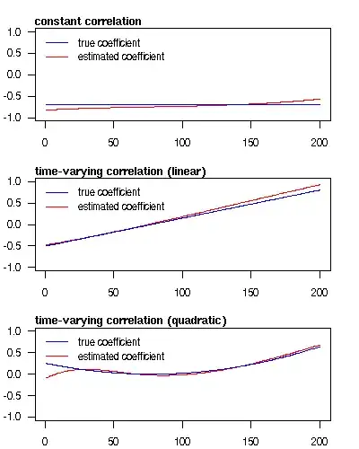
The plot can be reproduced with the following R code.
require(splines)
par(mfrow = c(1,3), mar = c(2, 2, 2, 2), las = 1, cex = 1.1, oma = c(1,1,1,1))

# example 1: the true coefficient is constant
set.seed(123)
n <- 200
x1 <- rnorm(n)
x2 <- -0.7 * x1 + rnorm(n, sd = 0.5)
Bspline <- bs(seq(0, 1, len = n), df=2)
fit <- lm(x2 ~ Bspline * x1)
summary(fit)
plot(seq_along(x1), coef(fit)[5] + Bspline %*% coef(fit)[6:8], ylim = c(-1, 1),
  xlab = "index", ylab = "", type = "l", col = "red")
lines(rep(-0.7, n), col = "blue")
legend("topleft", col = c("blue", "red"), legend = c("true coefficient", "estimated coefficient"),
  lty = c(1,1), bty = "n")
mtext(text = "constant correlation", side = 3, adj = 0, font = 2)

# example 2: the true coefficient follows a linear slope
set.seed(125)
n <- 200
x1 <- rnorm(n)
x2 <- seq(-0.5, 0.8, len=n) * x1 + rnorm(n, sd = 0.5)
Bspline <- bs(seq(0, 1, len = n), df=2)
fit <- lm(x2 ~ Bspline * x1)
summary(fit)
plot(seq_along(x1), coef(fit)[5] + Bspline %*% coef(fit)[6:8], ylim = c(-1, 1),
  xlab = "index", ylab = "", type = "l", col = "red")
lines(seq(-0.5, 0.8, len=n), col = "blue")
legend("topleft", col = c("blue", "red"), legend = c("true coefficient", "estimated coefficient"),
  lty = c(1,1), bty = "n")
mtext(text = "time-varying correlation (linear)", side = 3, adj = 0, font = 2)

# example 3: the true coefficient follows a quadratic form
set.seed(127)
n <- 200
x1 <- rnorm(n)
x2 <- (seq(-0.5, 0.8, len=n)^2) * x1 + rnorm(n, sd = 0.5)
Bspline <- bs(seq(0, 1, len = n), df=5)
fit <- lm(x2 ~ Bspline * x1)
summary(fit)
plot(seq_along(x1), coef(fit)[7] + Bspline %*% coef(fit)[8:12], ylim = c(-1, 1),
  xlab = "index", ylab = "", type = "l", col = "red")
lines(seq(-0.5, 0.8, len=n)^2, col = "blue")
legend("topleft", col = c("blue", "red"), legend = c("true coefficient", "estimated coefficient"),
  lty = c(1,1), bty = "n")
mtext(text = "time-varying correlation (quadratic)", side = 3, adj = 0, font = 2)
javlacalle
- 11,184
- 27
- 53
0
You could determine the correlation coefficient for subsets of time and then compare.
1-10 years 1-11 years 1-12 years ...and so on.
jack
- 139
- 1
- 4
0
A simple method would be to run moderated regression with time as the moderator. Center time and A then multiply them to create a product term. Using hier reg, enter A and time, then the product term. R2 change at the latter step shows mod effect of time on AB r.
Mr. Peabody
- 1
- 1
-
Following previous suggestion, you need to plot the slopes to confirm the direction of the moderation (strengthening or weakening over time). – Mr. Peabody Apr 11 '15 at 16:01