4

The aim is to estimate an error on a stochastic event rate dynamically.

This Question points in the same direction, I am interested in a theoretical extension.

I read out the event counter second-wise, every black $1$ is a counted event (new events over time, see the plot below).

During the measurement I am estimating the event rate, so as more statistics is accumulated, mean event rate (red) should asymptotically become more accurate.

dyn_mean1

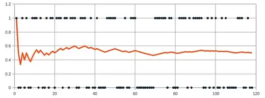
As one can see, the mean value oscillates around true value of 0.5,

dyn_mean2

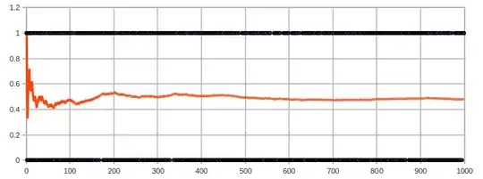
even after one order of magnitude more events collected.

Practical question: How can one calculate the number of events needed to estimate the mean value to a maximum error ($0.5\pm \sigma$)? - answered (?) here

Theoretical question: Can this oscillation be described analytically? Can you suggest further reading?

The events are radiation counts, so they are uncorrelated, may by Poisson-distribution applied?

Addendum: Idealized first approximation - every 10th event is non-zero: dyn_mean_reg1

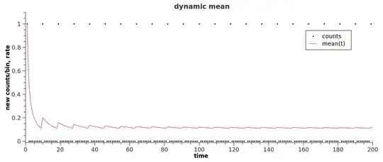
May be this curve is superimposed with the realer-life example above, is any techniques of partitioning in arbitrary functions applicable here?

IljaBek
  • 93
  • 6
  • See my comment to the referenced question. For the theoretical question, read about Brownian motion and random walks. – whuber Aug 19 '11 at 22:53

2 Answers2

5

This is an answer to your first "theoretical" question Can this oscillation be described analytically? Can you suggest further reading?

If I understand your question correctly, you are in the situation of independent identically distributed random variables with finite variance $\sigma^2$. In this case the law of the iterated logarithm applies which tells you that you should expect the difference between estimated mean and mean to oscillate between $-\sigma$ and $+\sigma$, if you normalize it by dividing by $\sqrt{2n\log{\log{n}}}$.

The linked wikipedia pages are good for a first reading. Wolfram offers a demo (which didn't work in my browser).

j.p.
  • 180
  • 4
  • 10
1

If you are estimating an unknown probability $p$, then, assuming i.i.d. nature of your events, the count $X$ is Binomial, with variance $np(1-p)$, where $n$ is the total number of events. The estimated proportion is $\hat p = X/n$ with variance $p(1-p)/n\le 0.5 \cdot 0.5 / n = 0.25/n$ for any $p$. For a given margin of error $m$, you can say that, approximately, $\mbox{Prob}[ |\hat p-p|>m ] \le \mbox{Prob}[ |Z|>m/(0.5/\sqrt{n}) ]$ where $Z$ is the standard normal variate. (You can do exact calculations with pbinom if you really need to.) For a 5% tail probability, we have $m/(0.5/\sqrt{n})=1.96$; $n=(1.96/2m)^2$, so for 3% accuracy, we have $n=(1.96/(2\cdot0.03))^2 = 1067$. This gives you an answer to an unrelated question: Why are polls always conducted for the sample size of 1000 or so? (Answer: to get this 3% accuracy with 95% confidence.)

You can of course approach this from the point of view of Bayesian updating with say a Jeffrey's prior $\propto [p(1-p)]^{-1/2}$ (i.e., $B(\frac12, \frac12)$ distribution), and getting your data in until variance of the posterior (also a Beta distribution) is small enough. The above derivation, essentially, assumes a flat prior, $B(1,1)$.

StasK
  • 29,235
  • 2
  • 80
  • 165