Random walk estimation with AR(1)

Question

When I estimate a random walk with an AR(1), the coefficient is very close to 1 but always less.

What is the math reason that the coefficient is not greater than one?

Answer 1

We estimate by OLS the model $$x_{t} = \rho x_{t-1} + u_t,\;\; E(u_t \mid \{x_{t-1}, x_{t-2},...\}) =0,\;x_0 =0$$

For a sample of size T, the estimator is

$$\hat \rho = \frac {\sum_{t=1}^T x_{t}x_{t-1}}{\sum_{t=1}^T x_{t-1}^2} = \rho + \frac {\sum_{t=1}^T u_tx_{t-1}}{\sum_{t=1}^T x_{t-1}^2}$$

If the true data generating mechanism is a pure random walk, then $\rho=1$, and

$$x_{t} = x_{t-1} + u_t \implies x_t= \sum_{i=1}^t u_i$$

The sampling distribution of the OLS estimator, or equivalently, the sampling distribution of $\hat \rho - 1$, is not symmetric around zero, but rather it is skewed to the left of zero, with $\approx 68$% of obtained values (i.e. $\approx$ probability mass) being negative, and so we obtain more often than not $\hat \rho < 1$. Here is a relative frequency distribution

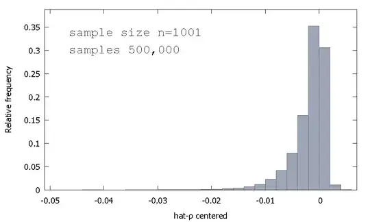
$$\begin{align} \text{Mean:} -0.0017773\\ \text{Median:} -0.00085984\\ \text{Minimum: } -0.042875\\ \text{Maximum: } 0.0052173\\ \text{Standard deviation: } 0.0031625\\ \text{Skewness: } -2.2568\\ \text{Ex. kurtosis: } 8.3017\\ \end{align}$$

This is sometimes called the "Dickey-Fuller" distribution, because it is the base for the critical values used to perform the Unit-Root tests of the same name.

I don't recollect seeing an attempt to provide intuition for the shape of the sampling distribution. We are looking at the sampling distribution of the random variable

$$\hat \rho - 1 = \left(\sum_{t=1}^T u_tx_{t-1}\right)\cdot \left(\frac {1}{\sum_{t=1}^T x_{t-1}^2}\right)$$

If $u_t$'s are Standard Normal, then the first component of $\hat \rho - 1$ is the sum of non-independent Product-Normal distributions (or "Normal-Product"). The second component of $\hat \rho - 1$ is the reciprocal of the sum of non-independent Gamma distributions (scaled chi-squares of one degree of freedom, actually).

For neither do we have analytical results so let's simulate (for a sample size of $T=5$).

If we sum independent Product Normals we get a distribution that remains symmetric around zero. For example:

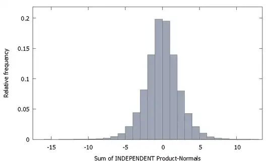
But if we sum non-independent Product Normals as is our case we get

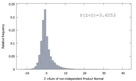
which is skewed to the right but with more probability mass allocated to the negative values. And the mass appears to being pushed even more to the left if we increase the sample size and add more correlated elements to the sum.

The reciprocal of the sum of non-independent Gammas is a non-negative random variable with positive skew.

Then we can imagine that, if we take the product of these two random variables, the comparatively greater probability mass in the negative orthant of the first, combined with the positive-only values that occur in the second (and the positive skewness which may add a dash of larger negative values), create the negative skew that characterizes the distribution of $\hat \rho -1$.

Answer 2

This is not really an answer but too long for a comment, so I post this anyway.

I was able to get a coefficient greater than 1 two times out of a hundred for a sample size of 100 (using "R"):

N=100                   # number of trials
T=100                   # length of time series
coef=c()
for(i in 1:N){
 set.seed(i)
 x=rnorm(T)             # generate T realizations of a standard normal variable
 y=cumsum(x)            # cumulative sum of x produces a random walk y
 lm1=lm(y[-1]~y[-T])    # regress y on its own first lag, with intercept
 coef[i]=as.numeric(lm1$coef[1])
}
length(which(coef<1))/N # the proportion of estimated coefficients below 1

Realizations 84 and 95 have coefficient above 1, so it is not always below one. However, the tendency is clearly to have a downward-biased estimate. The questions remains, why?

Edit: the above regressions included an intercept term which does not seem to belong in the model. Once the intercept is removed, I get many more estimates above 1 (3158 out of 10000) -- but still it is clearly below 50% of all the cases:

N=10000                 # number of trials
T=100                   # length of time series
coef=c()
for(i in 1:N){
 set.seed(i)
 x=rnorm(T)             # generate T realizations of a standard normal variable
 y=cumsum(x)            # cumulative sum of x produces a random walk y
 lm1=lm(y[-1]~-1+y[-T]) # regress y on its own first lag, without intercept
 coef[i]=as.numeric(lm1$coef[1])
}
length(which(coef<1))/N # the proportion of estimated coefficients below 1