7

I am currently working on a statistical project where I need to estimate a conditional expectation $E[Y|X=x_i]$ using the Nadaraya-Watson estimator. For doing that, I have the sample $(x_1,y_1),...,(x_n,y_n)$, where $n=14$, and I have chosen the bandwidth $h$ such that : $h = n^{-\frac{1}{5}}=0.5899$, given that the common rule of thumb is to have $h \propto n^{-\frac{1}{5}}$ for optimality.

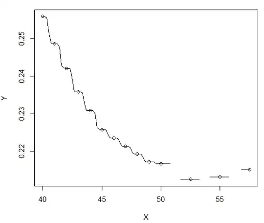
However, I do not get in what sense that $h$ is optimal. Indeed, I am using R, the ksmooth function with a normal kernel : ksmooth(X,Y,"normal",bandwidth=h).This is what I get if I choose such a $h$:

enter image description here

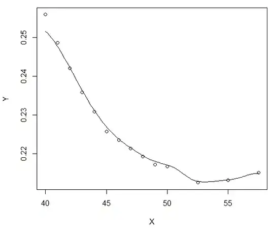
While if for example I choose $h$ equal to 3 (so around 5 times bigger), I get a way smoother curve, which is what really interests me:

enter image description here

Could someone explain me in what sense having $h \propto n^{-\frac{1}{5}}$ is "optimal"?

What am I sacrificing if I choose a $h$ bigger than the "optimal" one: accuracy, convergence speed, etc.?

I greatly appreciate, thank you very much.

JJFM
  • 81
  • 3
  • P.S. this is the second message I post in which my beginning "Hello everyone" is erased, does somebody know why? I wouldn't like to seem rude. – JJFM Mar 26 '15 at 18:27
  • Well, according to Bochner-Landau notation, both are equivalent big-O. In any case, you should not be computing the bandwidth by hand, but using a rule like Rupert-Sheather-Wand implemented in the `KernSmooth` package. – tchakravarty Mar 26 '15 at 19:17
  • Sorry T C, I don't get it, what is equivalent to what? The function you refer to from the `KernSmooth` package is `dpill`? The issue here is that my priority is smoothness, and if an optimal bandwidth yields a graph like the 1st one I posted above it is useless, that is why I was asking what do I sacrifice when I increase the bandwidth with respect to some optimal value. – JJFM Mar 26 '15 at 19:24
  • 5*0.5899 is the same as 0.5899. Please post your data in order to show the performance of different theoretically motivated bandwidth selection rules. – tchakravarty Mar 26 '15 at 20:17
  • The "Hellos" "Thanks!"es and "Appologies if..." do not contribute to, and in fact distract from questions and answers. Remember your questions here, and responses to them are a collaborative community legacy, not simply a conversation you are having on your own. So those social niceties that work well on, say, social networking sites and forums are inappropriate here. – Alexis Mar 26 '15 at 21:35
  • Oh, I though that 3 was an order higher than 0.5899 @T C. For the moment, after observing the poor results I got with 0.5899, I just tried different (higher) values for h. Thank you for the clarification @Alexis – JJFM Mar 27 '15 at 08:57

1 Answers1

3

It's optimal in that it minimized the mean (integrated) squared error for a data generating process as a function of some parameters and the sample size. The trick is that "proportional to" means there's an unknown factor multiplying $n^{-\frac{1}{5}}$.

There are various candidates that are more or less data-driven, but the simplest RoT bandwidth when using a second order kernel is $$h=\sigma_x \cdot n^{-\frac{1}{5}}.$$

See Li and Racine, Nonparametric Econometrics: Theory and Practice, bottom of p.66. Usually, one can do much better than this by using CV to pick $h$ instead.

amoeba
  • 93,463
  • 28
  • 275
  • 317
dimitriy
  • 31,081
  • 5
  • 63
  • 138
  • Ok, thank you @Dimitriy V. Masterov, just a clarification, the standard deviation in your comment is the one from my data? – JJFM Mar 27 '15 at 08:59
  • Well thank you, I've checked this and the result is way better, in fact the standard deviation times n to the power of -1/5 yields 3.0965 so the curve is quite smooth. – JJFM Mar 27 '15 at 09:24
  • @JJFM Yes, I added a link to GB with the text. – dimitriy Mar 27 '15 at 16:02
  • This is an excellent textbook. – dv_bn Apr 19 '16 at 21:13