Consider the following Deming model with independent replicates :
$$x_{i,j} \mid \theta_{i} \sim {\cal N}(\theta_{i}, \gamma_X^2), \quad y_{i,j} \mid \theta_{i} \sim {\cal N}(\alpha+\beta\theta_{i}, \gamma_Y^2), \\ i \in 1:I, \quad j \in 1:J,$$ all observations being independent, all parameters being unknown.
Let's fix the parameters and the design and write a function that simulates the data:
N <- 25  # number of groups
J <- 4  # number of repetitions within each group
theta0 <- 1:N  # true theta_i
gammaX0 <- sqrt(4);
lambda <- 1
gammaY0 <- sqrt(lambda)*gammaX0
alpha <- 0
beta <- 1
simulations <- function(){
  X <- Y <- array(NA,dim=c(N,J))
  for(i in 1:N){
    for(j in 1:J){
      X[i,j] <- rnorm(1,theta0[i],gammaX0)
      Y[i,j] <- rnorm(1,alpha+beta*theta0[i],gammaY0)
    }
  }
return(list(X=X,Y=Y))
}
set.seed(666)
sims <- simulations()
X <- sims$X; Y <- sims$Y
When the ratio $\lambda=\frac{\gamma_Y^2}{\gamma_X^2}$ is known, one can get good estimates of $\alpha$ and $\beta$ by considering only the group means $$ \bar{x}_{i\bullet} \sim {\cal N}(\theta_i, \gamma_X^2/J), \quad \bar{y}_{i\bullet} \sim {\cal N}(\alpha + \beta\theta_i, \gamma_Y^2/J)$$ and then by taking the maximum likelihood estimates:
MethComp::Deming(rowMeans(X), rowMeans(Y), vr=lambda)[1:2]
##  Intercept      Slope
## -0.3207636  1.0154527
On the other hand, the least-squares estimates:
coefficients(lm(rowMeans(Y)~rowMeans(X)))
## (Intercept) rowMeans(X)
##  0.04505284  0.98709755
are biased and unconsistent.
Now, using a Bayesian approach with the following naive and independent priors: $$ \gamma_X^2 \sim {\cal IG}(0^+,0^+), \qquad \gamma_Y^2 \sim {\cal IG}(0^+,0^+), \\ \theta_i \sim {\cal N}(0, \infty), \\ \alpha \sim {\cal N}(0, \infty), \qquad \beta \sim {\cal N}(0, \infty), $$ then the Bayesian estimates (posterior means or medians) of $\alpha$ and $\beta$ are close to the least-squares estimates. And I wonder why.
I know there is no reason to get a good coincidence between maximum likelihood estimates and Bayesian estimates by using "naive" non-informative priors, but I am surprised by the coincidence between the least-squares estimates and the Bayesian estimates. Is there an intuitive reason to expect this result ?
This is what I discovered using JAGS:
library(rjags)
modelfile <- "gibbs1.txt"
jmodel <- function(){
  for(i in 1:N){
    for(j in 1:J){
      X[i,j] ~ dnorm(theta[i], inv.gammaX2)
      Y[i,j] ~ dnorm(nu[i], inv.gammaY2)
    }
    theta[i] ~ dnorm(0, 0.00001)
    nu[i] <- alpha+beta*theta[i]
  }
  alpha ~ dnorm(0,0.001)
  beta ~ dnorm(0,0.001)
  #
  inv.gammaX2 ~ dgamma(0.01,0.01)
  inv.gammaY2 ~ dgamma(0.01,0.01)
  gammaX2 <- 1/inv.gammaX2
  gammaY2 <- 1/inv.gammaY2
  lambda <- gammaY2/gammaX2
}
writeLines(paste("model", paste(body(jmodel), collapse="\n"), "}"), modelfile)
# run Gibbs sampler
data <- list(X=X, Y=Y, N=N, J=J)
inits1 <- list(alpha=0, beta=1, inv.gammaX2=1, inv.gammaY2=1, theta=rowMeans(X))
inits2 <- lapply(inits1, function(x) x*rnorm(length(x),1,.01))
inits <- list(inits1,inits2)
jags <- jags.model(modelfile,
                   data = data,
                   inits=inits,
                   n.chains = 2,
                   n.adapt = 1000,
                   quiet=TRUE)
update(jags, 5000, progress.bar="none")
samples <- coda.samples(jags, c("alpha", "beta"), 10000, progress.bar="none")
summary(samples)$statistics
##              Mean         SD     Naive SE Time-series SE
## alpha -0.03753944 0.65340570 0.0046202760    0.016653968
## beta   0.99340104 0.04402299 0.0003112895    0.001129354
Below are the results of $1000$ simulations (I can provide the code for simulations) :
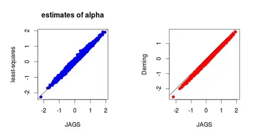
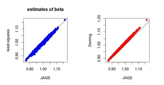
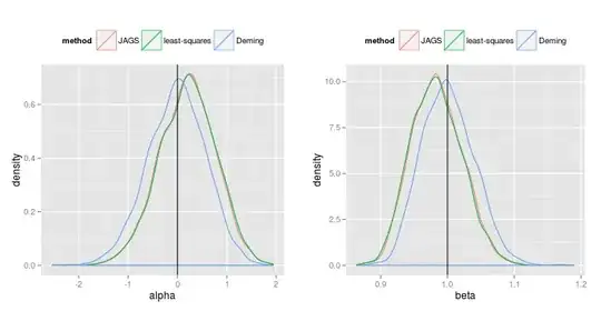
In fact, it is not difficult to derive the full conditional distributions in the Gibbs sampler. And one gets (I can provide details if needed):
the full conditional distribution of $\theta_i$ is a Gaussian distribution and the expression of its mean as a function of $(\alpha, \beta)$ is the same as the expression of the ML estimate of $\theta_i$ as a function of the ML estimates $(\hat\alpha, \hat\beta)$ assuming the known ratio $\lambda=\gamma^2_Y/\gamma_X^2$;
the full conditional distribution of $(\alpha, \beta)$ is a Gaussian distribution centered around the ML ($=$ least-squares) estimates for the ordinary regression of the $y_{ij}$ vs the $\theta_i$ (each $\theta_i$ replicated $J$ times).
It is interesting to note that iterating the above procedure about the means, by assuming the true ratio at first step, yields the maximum likelihood estimates:
alpha <- 0; beta <- 1 # initial values
for(iter in 1:100){
  theta <- rowMeans(X) + beta/(lambda+beta^2)*(rowMeans(Y)-(alpha+beta*rowMeans(X)))
  ab <- coefficients(lm(c(t(Y))~I(rep(theta, each=J))))
  alpha <- ab[1]; beta <- ab[2]
}
ab
##             (Intercept) I(rep(theta, each = J))
##              -0.3207636               1.0154527
MethComp::Deming(rowMeans(X), rowMeans(Y), vr=lambda)[1:2]
##  Intercept      Slope
## -0.3207636  1.0154527
In view of this fact I would be tempted to expect Bayesian estimates close to the maximum likelihood estimates, and not the least-squares estimates (corresponding to maximum likelihood estimates when $\lambda=\infty$). What is wrong in this intuition ?