Consider a simple time series:
> tp <- seq_len(10)
> tp
 [1]  1  2  3  4  5  6  7  8  9 10
we can compute an adjacency matrix for this time series representing the temporal links between samples. In computing this matrix we add an imaginary site at time 0 and the link between this observation and the first actual observation at time 1 is known as link 0. Between time 1 and time 2, the link is link 1 and so on. Because time is a directional process, sites are connected to (affected by) links that are "upstream" of the site. Hence every site is connected to link 0, but link 9 is only connected to site 10; it occurs temporally after each site except site 10. The adjacency matrix thus defined is created as follows:
> adjmat <- matrix(0, ncol = length(tp), nrow = length(tp))
> adjmat[lower.tri(adjmat, diag = TRUE)] <- 1
> rownames(adjmat) <- paste("Site", seq_along(tp))
> colnames(adjmat) <- paste("Link", seq_along(tp)-1)
> adjmat
        Link 0 Link 1 Link 2 Link 3 Link 4 Link 5 Link 6 Link 7
Site 1       1      0      0      0      0      0      0      0
Site 2       1      1      0      0      0      0      0      0
Site 3       1      1      1      0      0      0      0      0
Site 4       1      1      1      1      0      0      0      0
Site 5       1      1      1      1      1      0      0      0
Site 6       1      1      1      1      1      1      0      0
Site 7       1      1      1      1      1      1      1      0
Site 8       1      1      1      1      1      1      1      1
Site 9       1      1      1      1      1      1      1      1
Site 10      1      1      1      1      1      1      1      1
        Link 8 Link 9
Site 1       0      0
Site 2       0      0
Site 3       0      0
Site 4       0      0
Site 5       0      0
Site 6       0      0
Site 7       0      0
Site 8       0      0
Site 9       1      0
Site 10      1      1
The SVD provides a decomposition of this matrix into Eigenfunctions of variation as different temporal scales. The figure below shows the extracted functions (from SVD$u)
> SVD <- svd(adjmat, nu = length(tp), nv = 0)
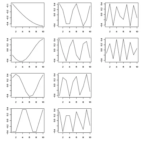
The eigenfunctions are periodic components at various temporal scales. Trying tp <- seq_len(25) (or longer) shows this better than the shorter example I showed above.
Does this sort of analysis have a proper name in statistics? It sounds similar to Singular Spectrum Analysis but that is a decomposition of an embedded time series (a matrix whose columns are lagged versions of the time series).
Background: I came up with this idea by modifying an idea from spatial ecology called Asymmetric Eigenvector Maps (AEM) which considers a spatial process with known direction and forming an adjacency matrix between a spatial array of samples that contains 1s where a sample can be connected to a link and a 0 where it can't, under the constraint that links can only be connected "downstream" - hence the asymmetric nature of the analysis. What I described above is a one-dimensional version of the AEM method. A reprint of the AEM method can be found here if you are interested.
The figure was produced with:
layout(matrix(1:12, ncol = 3, nrow = 4))
op <- par(mar = c(3,4,1,1))
apply(SVD$u, 2, function(x, t) plot(t, x, type = "l", xlab = "", ylab = ""),
      t = tp)
par(op)
layout(1)