Gung's answer is excellent, but I want to add an interpretation that I think goes underappreciated.
You wrote out the model as
$$
Y = \beta_0 + \beta_1 X_1 + \beta_2 X_2 + \varepsilon
$$
You didn't specify this, but presumably $\varepsilon$ is an error term with $\operatorname{\mathbb{E}}\left(\varepsilon\,|\,X\right) = 0$ and $\varepsilon \perp X$. Here you are postulating a particular data-generating process: given $X_1$ and $X_2$, $Y$ is a deterministic function of $X_1$ and $X_2$, plus a random error term. This is what is usually taught in undergrad econometrics class.
Now just for the heck of it, define a function $\mu(x_1, x_2) = \beta_0 + \beta_1 x_1 + \beta_2 x_2$ so that the model can be written as
$$
Y = \mu(X_1, X_2) + \varepsilon
$$
or, perhaps more precisely,
$$
Y\,|\,(X_1 = x_1, X_2 = x_2) = \mu(x_1, x_2) + \varepsilon
$$
Remember that we assumed $\operatorname{\mathbb{E}}\left(\varepsilon\,|\,X_1 = x_1, X_2 = x_2\right) = 0$. Taking the hint, let's compute
$$
\begin{align}
\operatorname{\mathbb{E}}(Y\,|\,X_1 = x_1, X_2 = x_2) &= \operatorname{\mathbb{E}}(\mu(x_1, x_2)) &+& \operatorname{\mathbb{E}}\left(\varepsilon\,|\,X_1 = x_1, X_2 = x_2\right) \\
\operatorname{\mathbb{E}}(Y\,|\,X_1 = x_1, X_2 = x_2) &= \mu(x_1, x_2) &+& 0 \\
\operatorname{\mathbb{E}}(Y\,|\,X_1 = x_1, X_2 = x_2) &= \beta_0 + \beta_1 x_1 + \beta_2 x_2
\end{align}
$$
This is powerful stuff: "regression line" is really the expected $Y$ as a function of $X$.
You asked what it means if $\beta_1 = 0$. In this interpretation, it means that the expectation of $Y$ does not depend on $X_1$. That is,
$$\begin{align}
\operatorname{\mathbb{E}}(Y\,|\,X_1 = x_1, X_2 = x_2) &= \beta_0 &+ 0 \cdot x_1 &+ \beta_2 x_2 \\
\operatorname{\mathbb{E}}(Y\,|\,X_1 = x_1, X_2 = x_2) &= \beta_0 &&+ \beta_2 x_2
\end{align}$$
In other words, $\beta_1 = 0$ means $X_1$ does not belong in the model. The slope of the regression line (i.e. the "conditional expectation line") is 0 with respect to $X_1$. Compare: $z = 2x + 2y$ and $z = 0x + 2y$
Now remember our second assumption that $\varepsilon \perp X$. From this we can conclude that in fact $Y \perp X_1$. We have already established that changing the value of $X_1$ has no effect on $\mu$, the average $Y$ given $X_1$ and $X_2$, but if $\varepsilon \perp X_1$ as well, then there's just nowhere else for $X_1$ to enter the data generating process. It doesn't affect the average $Y$ and it doesn't effect the variation of $Y$ around its average, so it just doesn't affect $Y$ at all.
Empirically, this means that any value we estimate for $\beta_1$, which we usually denote $\hat \beta_1$, should be close to zero. If we use OLS to fit the model, we know that $\operatorname{\mathbb{E}}(\hat \beta_1) = \beta_1 = 0$ and $\hat \beta_1 \xrightarrow[]{n \to \infty} \beta_1$. So the expectation of $\hat \beta_1$ will be zero, and $\hat \beta_1$ will approach zero as the sample grows.
