Predicting the growth of traffic on a web site: regression or time series?

Question

I've got a small website and I'm investing a lot of efforts on it. The traffic is growing but still very low. I've studied engineering but my knowledge of statistics is basic.

I have put the last 70 days of data on Google Doc (link) and I wish to detect daily seasonality, level shifts, time trends in a logical way while also identifying unusual readings and not have them distort my forecast. What method should I use?

I've tried Excel with a linear, logarithmic regression. Are these forecast statistically reliable?

What is an alternative for this kind of task? (i.e. other type of regression? time series?)

Answer 1

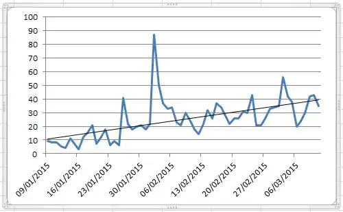
Statistics can be loosely defined as the practice of converting data to information. The original data may have "unusual" i.e. non-typical values that often obfuscate the routine identification of a useful model. The idea here is to separate the data into signal and error i.e.deviations from the signal. Now these deviations can often be divided into typical deviations and exceptional deviations. The "cause" of the exceptional deviations can reflect one-time anomalies , seasonal anomalies and/or level shifts/time trends reflecting a set of consistent anomalies. Intervention Detection schemes suggested by many including http://www.unc.edu/~jbhill/tsay.pdf and http://www.autobox.com/cms/index.php/blog/entry/build-or-make-your-own-arima-forecasting-model enable the identification of "exceptional deviations". If we however review the graph of the 70 daily values we immediately can suggest that 4 values (days 26,33,34 and 62 ) may be candidates for possible adjustment prior to model identification:

The plot of the original data is !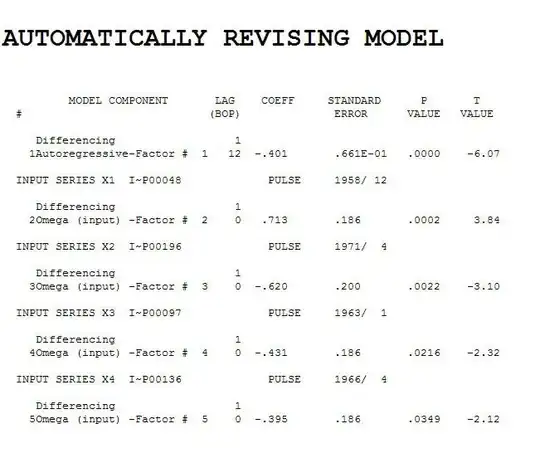

day actual adjusted;;;

26 48 19 ; 33 87 36 ; 34 50 36 ; 62 56 38 ;

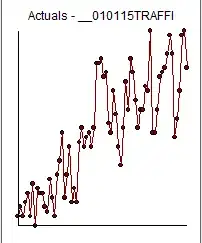
This step can of course be automated but for our discussion here I will simply suggest for purposes of education a step-by-step approach. A plot of the outlier-adjusted data is . Now if we compute the acf of this adjusted data we obtain suggesting that a simple ARIMA (1,0,0)(0,0,0) might be appropriate ( N.B. this was further suggested by the PACF showing a spike at lag 1 ). If we proceed to estimate this ARIMA model in a robust manner we obtain 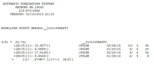an AR(1) with 4 pulses for these 70 values.

We now inspect the acf of the residuals from this model and obtain what perhaps might be clues/evidence of either a sufficient model or a model needing further tweaking/augmentation.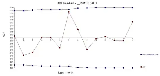 suggesting the need to either add a seasonal ar component (stochastic) culminating in (1,0,0)(1,0,0)7 OR adding seasonal/daily dummies to reflect a deterministic component. Diagnostic checking in a manual i.e. non-automatic manner as to which remedy is best requires simply trying both ways. If we use the seasonal ar augmentation we obtain the following model with actual/fit/forecast 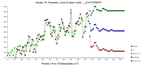. If we chose a model that contains a set of daily dummies 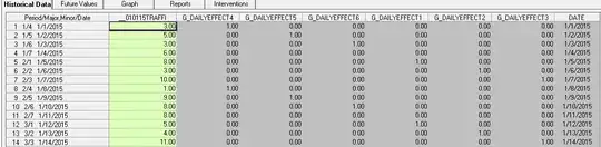to characterize the seasonal/daily effect we obtain the following model 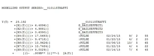with actual/fit/forecast 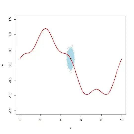. The statistics suggest that either model may be adequate suggesting that both should be considered. In closing the totally automatic solution (not shown here) preferred the second approach. Model identification using one statistic like the AIC/BIC simply doesn't due justice to the intelligent design of model form,but that is just my opinion. Recall all models are wrong but these two final models seem useful. Note also the fairly broad confidence limits suggesting possibly a different level.

RE: Nick's comment

@NickCox The ar(1) term and the constant generate a long term assymptotic forecast comimg off recent values to a constant. Note that the mean of the last 38 values is 30.1 reflecting a significantly different (higher) mean from the first 32 but not suggesting continued growth. In the case of the AR(1) with the model with the three daily dummies the sum of the next 30 forecasts is 861 for an average of 28 sympathetic to and not significantly different the 30.1 . I definitely think that this is not the only model that could be used for this data.