I will demonstrate using an AR(1) model. Consider a variable, $\left(y_{t}\right)_{t=0,1,\ldots}
$. Then consider the AR(1) model: $y_{t}=\rho y_{t-1}+\varepsilon_{t},\quad\varepsilon_{t}\thicksim N\left(0,\,\sigma^{2}\right)
$.
Solving the AR(1) model we get:$y_{t}=\rho^{t}y_{0}+\sum_{i=0}^{t-1}\rho^{i}\varepsilon_{t-i}
$
where $y_{0}
$ is the initial value of the process. Finding the variance we get: $\sigma^{2}\frac{1-\rho^{2t}}{1-\rho}
$. Clearly this process is not stationary nor weakly mixing (hence its not ergodic since weakly mixing imlies ergodicity) as both the conditional mean and the conditional variance depend upon time. We can therefore write:$y_{t}=\rho^{t}y_{0}+\sum_{i=0}^{t-1}\rho^{i}\varepsilon_{t-i}\stackrel{D}{=}N\left(\rho^{t}y_{0},\,\sigma^{2}\frac{1-\rho^{2t}}{1-\rho^{2}}\right)
$
If however the condition $\left|\rho\right|<1
$ holds then the series is stationary and weakly mixing (hence ergodic since weakly mixing implies ergodicity) and we can write it as:$y_{t}=\sum_{i=0}^{t-1}\rho^{i}\varepsilon_{t-i}\stackrel{D}{=}N\left(0,\,\sigma^{2}\frac{1}{1-\rho^{2}}\right)
$
since when $\left|\rho\right|<1
$ holds then $\rho^{t}\rightarrow0
$ exponentially fast and we have that $\rho^{t}y_{0}\rightarrow0
$ and $\sigma^{2}\frac{1-\rho^{2t}}{1-\rho^{2}}\rightarrow\sigma^{2}\frac{1}{1-\rho^{2}}
$ exponentially fast. To summarize, when $\left|\rho\right|<1$
and $\varepsilon_{t}$
is normally distributed then the condition $\left|\rho\right|<1$
is enough to ensure ergodicity of both the mean and the variance. Now we know that $\left|\rho\right|<1
$ is enough to ensure stationarity and ergodicity of the AR(1) process and in order to test this we could run a unit root test on the series and see if the series had a unit root or not. Other sources of non-stationarity could be a deterministic trend, changing variance and structural breaks, all of which we could model. A unit root however needs a transformation of the data or we could use cointegration analysis if we had more than one series.
To illustrate I will simulate the AR(1) model: $y_{t}=y_{t-1}+\varepsilon_{t}
$:
We see that the autocorrelation function decays very slowly and from the time series graph the series does not look very stationary. Therefore we can say that clearly the assumption about stationarity and weakly mixing (hence ergodicity) does not hold when $\left|\rho\right|=1
$. For information about the autocorrelation function see here.
For the second illustration I will simulate the AR(2), $y_{t}=0.3y_{t-1}+0.4y_{t-1}+\varepsilon_{t}
$ model but I will try to model it with an AR(1) model to see how the residuals look like.
We see that the time series graph looks stationary and the ACF goes exponentially towards zero indicating stationarity and weakly mixing. By fitting an AR(1) model to the data we get the following model: $y_{t}=0.54y_{t-1}+\varepsilon_{t}
$. If we now look at the residual ACF we see that they are not white noise (a martingale diff. seq. is white noise) and the portmanteu test rejects the null of no autocorrelation.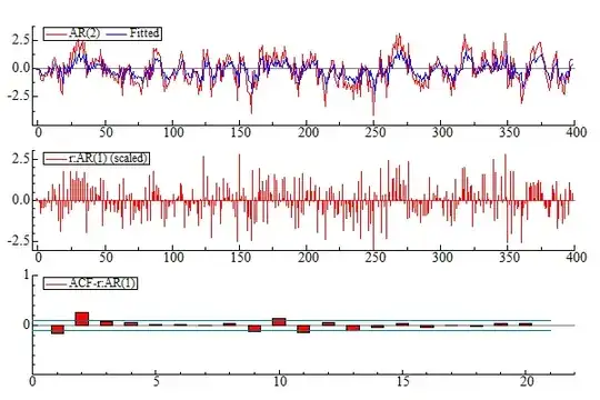
If we then fit an AR(2) to the simulated data we get an estimated model of: $y_{t}=0.37y_{t-1}+0.32y_{t-1}+\varepsilon_{t}
$. Now the residuals do look like white noise and we cannot reject the null of no autocorrelation.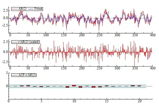
If this did not answer your question then let me know.