This is related to equating (e.g. here). In the case of equating you take two variables $X$ and $Y$ (e.g. two tests taken by a single group of students) and transform the distribution of $X$ in such a way that it resembles the distribution of $Y$. If you want to preserve only the first two moments you could use linear equating:
$$ \operatorname{Lin}_Y(x_i) = \frac{\sigma_Y}{\sigma_X}x_i + \left( \mu_Y - \frac{\sigma_Y}{\sigma_X}\mu_X \right) $$
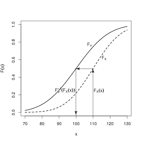
However if you want to be more precise and match the quantiles, then a little bit more advanced method is needed, i.e. equipercentile equating, where you use cumulative distribution functions and their inverses of $X$ and $Y$:
$$ \operatorname{Equi}_Y(x_i) = F^{-1}_Y \left[ F_X(x_i) \right] $$
So the general idea is that you can find such values $u_i$ that range from $0$ to $1$ that correspond to certain values of $F_X(x_i)$ and then find values of $F_Y(y_i)$ that correspond to those values:
$$ F_X(x_i) = u_i = F_Y(y_i) $$
Of course this works only for continuous data, so with discrete data you need an additional step - "smoothing" of data. For this purpose kernel smoothing is often used.
Below you can find an example of R library that implements those methods (req4 from example(equate)). Empirical distribution x is transformed to match y, where yx is the outcome. As you can see, resulting mean, standard deviation, skewness and kurtosis of the outcome are close to the target.
Equipercentile Equating: rx to ry

Design: equivalent groups

Smoothing Method: loglinear presmoothing

Summary Statistics:
    mean   sd skew kurt  min   max    n
x  19.85 8.21 0.38 2.30 1.00 40.00 4329
y  18.98 8.94 0.35 2.15 1.00 40.00 4152
yx 18.98 8.99 0.35 2.21 0.01 40.05 4329