When I launch this code (sorry, I cannot post my data):
fc3 <- avgScore ~ slope_mean + water_dist + clc_231 + clc_242 + clc_321
mc3 <- lm(fc3, data = d)
require(car)
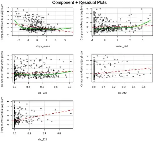
residualPlot(mc3)
I get the following plot:
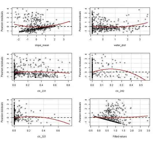
What is confusing is that the first residual plot of the slope_mean suggest there is positive relationship of slope_mean with the response variable. But in fact the relationship is negative:
> summary(mc3)

Call:
lm(formula = fc3, data = d)

Residuals:
    Min      1Q  Median      3Q     Max
-1.6643 -0.6329 -0.3172  0.2015  4.0340

Coefficients:
            Estimate Std. Error t value      Pr(>|t|)
(Intercept)  0.43228    0.07667   5.638 0.00000002991 ***
slope_mean  -0.33510    0.05455  -6.143 0.00000000174 ***
water_dist   0.07266    0.05435   1.337      0.181930
clc_231      0.61033    0.28698   2.127      0.033972 *
clc_242      2.28195    0.64049   3.563      0.000405 ***
clc_321      2.95934    0.66945   4.421 0.00001226661 ***
---
Signif. codes:  0 ‘***’ 0.001 ‘**’ 0.01 ‘*’ 0.05 ‘.’ 0.1 ‘ ’ 1

Residual standard error: 1.046 on 465 degrees of freedom
Multiple R-squared:  0.1502,    Adjusted R-squared:  0.1411
F-statistic: 16.44 on 5 and 465 DF,  p-value: 5.991e-15
When I try to create the first plot by hand, as I understand the residual plot, I get something else:
# do the same model without the first variable and take its residuals
fc3r <- avgScore ~ water_dist + clc_231 + clc_242 + clc_321
mc3r <-  lm(fc3r, data = d)

x <- d$slope_mean
y <- resid(mc3r)

plot(x, y)

spl1 <- smooth.spline(x, y, tol = 1e-6, df = 8)
lines(spl1, col = "red", lwd = 2)
I get the plot below, which is pretty much different from the first residual plot above. In this plot it looks like the slope of the densiest cluster is 0, while in the above residual plots it looks like the slope is positive. So did I understand and reconstruct the partial residual plots wrong?
EDIT: note that with crPlot I get different residual plot, more similar to mine one, but not the same (this makes it even more messy):