Intuition behind why Stein's paradox only applies in dimensions $\ge 3$

Question

Stein's Example shows that the maximum likelihood estimate of $n$ normally distributed variables with means $\mu_1,\ldots,\mu_n$ and variances $1$ is inadmissible (under a square loss function) iff $n\ge 3$. For a neat proof, see the first chapter of Large-Scale Inference: Empirical Bayes Methods for Estimation, Testing, and Prediction by Bradley Effron.

This was highly surprising to me at first, but there is some intuition behind why one might expect the standard estimate to be inadmissible (most notably, if $x \sim \mathcal N(\mu,1)$, then $\mathbb{E}\|x\|^2\approx \|\mu\|^2+n$, as outlined in Stein's original paper, linked to below).

My question is rather: What property of $n$-dimensional space (for $n\ge 3$) does $\mathbb{R}^2$ lack which facilitates Stein's example? Possible answers could be about the curvature of the $n$-sphere, or something completely different.

In other words, why is the MLE admissible in $\mathbb{R}^2$?

---

Edit 1: In response to @mpiktas concern about 1.31 following from 1.30:

$$E_\mu\left(\|z-\hat{\mu}\|^2\right)=E_\mu\left(S\left(\frac{N-2}{S}\right)^2\right)=E_\mu\left(\frac{(N-2)^2}{S}\right).$$

$$\hat{\mu_i} = \left(1-\frac{N-2}{S}\right)z_i$$ so $$E_\mu\left(\frac{\partial\hat{\mu_i}}{\partial z_i} \right)=E_\mu\left( 1-\frac{N-2}{S}+2\frac{z_i^2}{S^2}\right).$$ Therefore we have:

$$2\sum_{i=1}^N E_\mu\left(\frac{\partial\hat{\mu_i}}{\partial z_i} \right)=2N-2E_\mu\left(\frac{N(N-2)}{S}\right)+4E_\mu\left(\frac{(N-2)}{S}\right)\\=2N-E_\mu\frac{2(N-2)^2}{S}.$$

Edit 2: In this paper, Stein proves that the MLE is admissible for $N=2$.

Answer 1

The dichotomy between the cases $d < 3$ and $d \geq 3$ for the admissibility of the MLE of the mean of a $d$-dimensional multivariate normal random variable is certainly shocking.

There is another very famous example in probability and statistics in which there is a dichotomy between the $d < 3$ and $d \geq 3$ cases. This is the recurrence of a simple random walk on the lattice $\mathbb{Z}^d$. That is, the $d$-dimensional simple random walk is recurrent in 1 or 2 dimensions, but is transient in $d \geq 3$ dimensions. The continuous-time analogue (in the form of Brownian motion) also holds.

It turns out that the two are closely related.

Larry Brown proved that the two questions are essentially equivalent. That is, the best invariant estimator $\hat{\mu} \equiv \hat{\mu}(X) = X$ of a $d$-dimensional multivariate normal mean vector is admissible if and only if the $d$-dimensional Brownian motion is recurrent.

In fact, his results go much further. For any sensible (i.e., generalized Bayes) estimator $\tilde{\mu} \equiv \tilde{\mu}(X)$ with bounded (generalized) $L_2$ risk, there is an explicit(!) corresponding $d$-dimensional diffusion such that the estimator $\tilde{\mu}$ is admissible if and only if its corresponding diffusion is recurrent.

The local mean of this diffusion is essentially the discrepancy between the two estimators, i.e., $\tilde{\mu} - \hat{\mu}$ and the covariance of the diffusion is $2 I$. From this, it is easy to see that for the case of the MLE $\tilde{\mu} = \hat{\mu} = X$, we recover (rescaled) Brownian motion.

So, in some sense, we can view the question of admissibility through the lens of stochastic processes and use well-studied properties of diffusions to arrive at the desired conclusions.

References

1. L. Brown (1971). Admissible estimators, recurrent diffusions, and insoluble boundary value problems. Ann. Math. Stat., vol. 42, no. 3, pp. 855–903.
2. R. N. Bhattacharya (1978). Criteria for recurrence and existence of invariant measures for multidimensional diffusions. Ann. Prob., vol. 6, no. 4, 541–553.

Answer 2

@cardinal gave a great answer (+1), but the whole issue remains mysterious unless one is familiar with the proofs (and I am not). So I think the question remains as to what is an intuitive reason that Stein's paradox does not appear in $\mathbb R$ and $\mathbb R^2$.

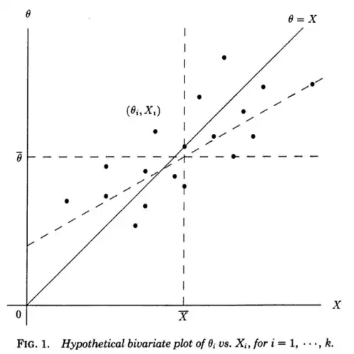
I find very helpful a regression perspective offered in Stephen Stigler, 1990, A Galtonian Perspective on Shrinkage Estimators. Consider independent measurements $X_i$, each measuring some underlying (unobserved) $\theta_i$ and sampled from $\mathcal N(\theta_i, 1)$. If we somehow knew the $\theta_i$, we could make a scatter plot of $(X_i, \theta_i)$ pairs:

The diagonal line $\theta = X$ corresponds to zero noise and perfect estimation; in reality the noise is non-zero and so the points are displaced from the diagonal line in horizontal direction. Correspondinly, $\theta = X$ can be seen as a regression line of $X$ on $\theta$. We, however, know $X$ and want to estimate $\theta$, so we should rather consider a regression line of $\theta$ on $X$ -- which will have a different slope, biased horizontally, as shown on the figure (dashed line).

Quoting from the Stigler's paper:

This Galtonian perspective on the Stein paradox renders it nearly transparent. The "ordinary" estimators $\hat \theta_i^0 = X_i$ are derived from the theoretical regression line of $X$ on $\theta$. That line would be useful if our goal were to predict $X$ from $\theta$, but our problem is the reverse, namely to predict $\theta$ from $X$ using the sum of squared errors $\sum (\theta_i - \hat \theta_i)^2$ as a criterion. For that criterion, the optimum linear estimators are given by the least squares regression line of $\theta$ on $X$, and the James-Stein and Efron-Morris estimators are themselves estimators of that optimum linear estimator. The "ordinary" estimators are derived from the wrong regression line, the James-Stein and Efron-Morris estimators are derived from approximations to the right regression line.

And now comes the crucial bit (emphasis added):

We can even see why $k\ge 3$ is necessary: if $k=1$ or $2$, the least squares line of $\theta$ on $X$ must pass through the points $(X_i, \theta_i)$, and hence for $k=1$ or $2$, the two regression lines (of $X$ on $\theta$ and of $\theta$ on $X$) must agree at each $X_i$.

I think this makes it very clear what is special about $k=1$ and $k=2$.