Edit: I found a solution to the problem, which is at the bottom of the post. I'm going to leave the post as it is in case someone else encounters a similar problem!
I was banging my head to a solution to the problem in the title and came up with a solution that partly works, but I'm not really happy with the result. With the algorithm I will outline I do generate a distribution with the input median and intervals, but the shape is definetly wrong. Let me explain:
The problem
In my field, it is typical to use Markov Chain Monte Carlo (MCMC) algorithms in order to generate posterior samples for parameters of highly non-linear models given the data.
For reasons I don't yet understand, although it is custom to generate MCMC samples for the posteriors, it is not custom for the authors to share those posterior distributions but, instead, some summary statistics on the posterior samples of the parameters given the data are published; the most common of which is to share the median and the "$1\sigma$" limits around the median, which usually means that, if $\theta$ is the parameter of interest and we denote its median by $\mu$, then the published value $\mu^{+\sigma_1}_{-\sigma_2}$ means that
$$\int^{\mu+\sigma_1}_{\mu} p(\theta | D) = 0.34,$$
$$\int^{\mu}_{\mu-\sigma_2} p(\theta | D) = 0.34,$$
where $p(\theta | D)$ is the posterior distribution of the parameter $\theta$ given the data $D$.
The problem is that I need to sample from those posterior distributions, so I tried to come up with an efficient idea on how to sample from a skewed distribution given the values of the median ($\mu$) and the upper and lower "1-sigma" limits ($\sigma_1$ and $\sigma_2$).
Proposed solution
After some thought, I came to the following conclusion: if I draw a sample from this posterior, I have an equal probability ($1/2$) of sampling a point to the left and to the right of the median. If for some reason I want to sample a point to the left of the median, then I have two parameters to do so: a location parameter ($\mu$) and a scale parameter ($\sigma_2$), while the same applies if I sample a point to the right of the median. Given a location and scale parameter, the safest choice seems to be to draw samples from a gaussian distribution. Thus, I came up with the following algorithm:
- Flip a coin (i.e., pick a number at random from the set $\Omega: \{0,1\})$.
- If heads (i.e., you got $0$ from the set $\Omega$), then sample a value from the distribution $X\sim N(0,\sigma_1)$, and let $Y = |X|$. If tails, sample a value from the distribution $X\sim N(0,\sigma_2)$, and let $Y = - |X|$
- Samples from the target distribution are given by $Z = \mu + Y$.
A small python code to sample $n$ points from this distribution would be as follows:
def sample_from_errors(mu, sigma1, sigma2, n):
    # Flip n coins (0 = heads; sample from right gaussian, 1: tails; sample from left gaussian):
    coin_flip = np.random.random_integers(0,1,n)
    # Extract which of those are heads and the number of them:
    idx_heads = np.where(coin_flip==0)[0]
    n_heads = len(idx_heads)
    # Extract samples from the left gaussian:
    samples_left_gaussian = mu - np.abs(np.random.normal(0,sigma2,n-n_heads))
    # Same for the right one:
    samples_right_gaussian = mu + np.abs(np.random.normal(0,sigma1,n_heads))
    return np.append(samples_left_gaussian,samples_right_gaussian)
Same, in R:
sample_from_errors <- function(mu, sigma1, sigma2, n){

 # Flip n coins (0 = heads; sample from right gaussian, 1: tails; sample from left gaussian):
 coin_flip <- sample(c(0,1), n, replace = TRUE)
 # Extract which of those are heads and the number of them:
 n_heads = n-sum(coin_flip)
 # Extract samples from the left and right gaussians:
 samples_left_gaussian = mu - abs(rnorm(n-n_heads, mean = 0, sd = sigma2))
 samples_right_gaussian = mu + abs(rnorm(n_heads, mean = 0, sd = sigma1))
 return (c(samples_left_gaussian,samples_right_gaussian))

}
Does it work?
The thing is that the above mentioned algorithm does work, in the sense that if you generate samples using the algorithm and calculate the median and $1-\sigma$ limits as defined in the introduction to this problem, you retrieve the original input values. The problem is the shape of the distribution that you get. For example, if you plot the histogram given $\mu = 10$, $\sigma_1 = 2$ and $\sigma_2 = 10$, you get the following ($n=10^6$ in this case):
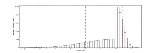
(Red solid line is the input median, red dashed lines the $1-\sigma$ limits) You can clearly see that the heights of the values in the histograms are different around sampled values of ~10 (close to the input median) which makes total sense: the heights of the gaussians that I'm sampling from ($1/\sqrt{2\pi \sigma_i^2}$) are variance dependent, and that explains the different heights at each side; the lower the variance, the greater the height of the distribution.
One way to solve this would be to resample the right side of the distribution in order to match the left sides' height, but that would change the lower $1-\sigma$ limit and, thus, kill the whole purpose of the algorithm.
What other methods have I tried?
(This method didn't work in my original post due to a mistake I made in the optimization code. It now works nicely!)
I tried fitting skew-normal distributions given the CDFs values that I'm looking for (i.e., parametrize given the 0.15866, 0.5 and 0.84134 quantiles), and this works fine now. Here is some python code that attempts at trying to perform this:
import numpy as np
from scipy.integrate import quad
from scipy.optimize import leastsq

def skew_normal_cdf(x,mu,sigma,alpha):
    """
    This function simply calculates the CDF at x given the parameters
    mu, sigma and alpha of a Skew-Normal distribution. It takes values or
    arrays as inputs.
    """
    # In case the input x is an array:
    if type(x) is np.ndarray:
       out = np.zeros(len(x))
       for i in range(len(x)):
           # quad calculates the integral from -inf to x[i]:
           out[i] = quad(lambda x: skew_normal(x,mu,sigma,alpha), -np.inf, x[i])[0]
       return out

    else:
        return quad(lambda x: skew_normal(x,mu,sigma,alpha), -np.inf, x)[0]

def skew_normal(x, mu, sigma, alpha):
    """
    This function returns the value of the Skew Normal PDF at x, given
    mu, sigma and alpha
    """
    def erf(x):
        # save the sign of x
        sign = np.sign(x)
        x = abs(x)

        # constants
        a1 =  0.254829592
        a2 = -0.284496736
        a3 =  1.421413741
        a4 = -1.453152027
        a5 =  1.061405429
        p  =  0.3275911

        # A&S formula 7.1.26
        t = 1.0/(1.0 + p*x)
        y = 1.0 - (((((a5*t + a4)*t) + a3)*t + a2)*t + a1)*t*np.exp(-x*x)
        return sign*y

    def palpha(y,alpha):
        phi = np.exp(-y**2./2.0)/np.sqrt(2.0*np.pi)
        PHI = ( erf(y*alpha/np.sqrt(2)) + 1.0 )*0.5
        return 2*phi*PHI

    return palpha((x-mu)/sigma,alpha)*(1./sigma)

def fit_skew_normal(median,sigma1,sigma2):

    # Define the sign of alpha, which should be positive if right skewed
    # and negative if left skewed:
    alpha_sign = np.sign(sigma1-sigma2)

    """
    This function is an attempt to fit a Skew Normal distribution given
    the median, upper error bars (sigma1) and lower error bar (sigma2).
    """

    # First, define the residuals:
    def residuals(p, data, x):
        mu, sqrt_sigma, sqrt_alpha = p
        return y - model(x, mu, sqrt_sigma, sqrt_alpha)

    # Now define the model:
    def model(x, mu, sqrt_sigma, sqrt_alpha):
        """
        Model for the non-linear least-squares problem.

        Note that we pass the square-root of the scale (sigma) and shape (alpha) parameters,
        in order to define the sign of the former to be positive and of the latter to be fixed given
        the values of sigma1 and sigma2:
        """
        return skew_normal_cdf (x, mu, sqrt_sigma**2, alpha_sign * sqrt_alpha**2)

    # Define the observed quantiles:
    y = np.array([0.15866, 0.5, 0.84134])

    # Define the values at which we observe the quantiles:
    x = np.array([median - sigma2, median, median + sigma1])

    # Start assuming that mu = median, sigma = mean of the observed sigmas, and alpha = 0 (i.e., start from a gaussian):
    guess = (median, np.sqrt ( 0.5 * (sigma1 + sigma2) ), 0)

    # Perform the non-linear least-squares optimization:
    plsq = leastsq(residuals, guess, args=(y, x))[0]

    # Return the fitted parameters of the Skew Normal (mu, sigma and alpha):
    return plsq[0], plsq[1]**2, alpha_sign*plsq[2]**2

# Just to test the code, generate first a set of parameters observed medians, sigma1 and sigma2:
median = 10.
sigma1 = 2.
sigma2 = 10.

# Now try and search for the Skew Normal distribution that matches those
# values:
plsq = fit_skew_normal(median,sigma1,sigma2)

# Print fitted values:
print 'Fitted params:',plsq
In this case, this code gives:
Fitted params: (14.70, 9.01, -28.25)
And the associated plot is:
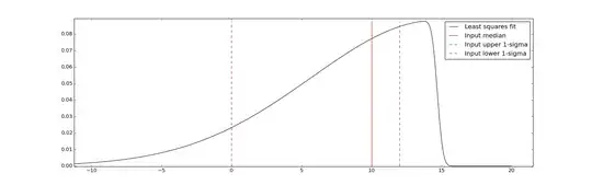
Which is good enough for my purposes I think!