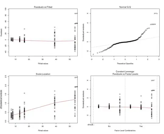
How do I read this linear model output from R?

Question

I normally use SPSS for my statistics, however after having some issues with violations I've had to try and run a linear model in R as apparently its more robust. Someone sent me the code that I should use. The issue is I can't make heads or tails of the output!

Can anyone help me?

> mouseData <- data.frame(mouse = factor(rep(c(1:36), each = 6)),
+                          shock = rep(factor(rep(c("No", "Yes"), each = 18)), 6),
+                          noise = rep(factor(c(75, 105, 115)), each = 72),
+                          day = rep(rep(factor(c(3, 29)), each = 36), each = 1), 
+ response = c(8.05,6.45,7.55,4.8,8.2,5.05,9.55,8.9,6.05,9.55,6.5,5.25,10.2,6,4.1,5.2,8.4,3.9,8.3,14.35,8.8,11.45,11.3,6.95,14.2,10.1,5.65,6.5,7.1,7.45,6.65,6.4,4.85,7.6,7.75,6.45,5.7,12.3,8.75,5.45,10.25,5.6,7.2,13.7,6.3,5.4,4.1,6.25,6.25,5.8,7.9,4.05,6,7.75,12.2,6.3,8.3,8.9,9.3,3.1,11.95,6.6,6.35,8.4,7.65,5.4,8.5,4.35,8.85,5.55,12.3,5.2,12.05,18.55,7.8,22,12.4,8.55,8.9,13.35,21.6,12.4,16.8,9.3,11.5,14.2,12.25,12.3,16.4,15.5,19.2,17.4,9.45,11.7,11.35,11.95,11.45,8,10.4,14.4,22.3,12.3,15.5,20.8,14.2,18.6,12.2,9.9,12.65,12.85,11.65,22.7,14.2,9.55,12.15,15.4,16.2,8.6,7.5,17.4,10.4,6.45,12.85,11.7,11.1,15.85,32.8,9.8,16.4,9.2,11,15.8,32.9,18.7,30.25,13.9,52,23.6,15.85,9.7,11.7,12.15,20.7,13.2,19.7,50.9,14.75,64.85,19.55,11.5,30.75,26.4,61.9,22.55,51.95,39.65,37.6,37.7,52.1,63.4,51.6,70.9,81.95,62.95,27.65,31.15,45.05,55.7,30.8,29.6,55.1,46.2,55.05,37.1,59.2,93.55,83.55,61.75,41.85,34.45,22.45,18.1,27.45,62.85,61.5,22.9,37.9,25,80.05,28.75,39.25,26.95,57.55,43.15,20.35,43.7,25.7,31.4,95.45,67.2,37.65,34.85,28.95,89.45,56.75,16.05,139.6,20.3,106.85,46.85,106.55,46.1,44.65,22.2,23.7,24.55))
> lm(response ~ shock * noise * day, data = mouseData)

Call:
lm(formula = response ~ shock * noise * day, data = mouseData)

Coefficients:
            (Intercept)                 shockYes                 noise105                 noise115  
                 6.8722                   1.5639                   6.7861                  33.5583  
                  day29        shockYes:noise105        shockYes:noise115           shockYes:day29  
                 0.2806                  -1.2722                   9.8194                  -0.9833  
         noise105:day29           noise115:day29  shockYes:noise105:day29  shockYes:noise115:day29  
                -1.2056                  -3.2111                   7.3833                   8.0833  

> mouseModel <- lm(response ~ shock * noise * day, data = mouseData)
> summary(mouseModel)

Call:
lm(formula = response ~ shock * noise * day, data = mouseData)

Residuals:
    Min      1Q  Median      3Q     Max 
-39.933  -4.190  -1.010   3.123  83.617 

Coefficients:
                        Estimate Std. Error t value Pr(>|t|)    
(Intercept)               6.8722     3.4644   1.984   0.0486 *  
shockYes                  1.5639     4.8994   0.319   0.7499    
noise105                  6.7861     4.8994   1.385   0.1675    
noise115                 33.5583     4.8994   6.849 8.56e-11 ***
day29                     0.2806     4.8994   0.057   0.9544    
shockYes:noise105        -1.2722     6.9288  -0.184   0.8545    
shockYes:noise115         9.8194     6.9288   1.417   0.1580    
shockYes:day29           -0.9833     6.9288  -0.142   0.8873    
noise105:day29           -1.2056     6.9288  -0.174   0.8620    
noise115:day29           -3.2111     6.9288  -0.463   0.6435    
shockYes:noise105:day29   7.3833     9.7988   0.753   0.4520    
shockYes:noise115:day29   8.0833     9.7988   0.825   0.4104    
---
Signif. codes:  0 ‘***’ 0.001 ‘**’ 0.01 ‘*’ 0.05 ‘.’ 0.1 ‘ ’ 1

Residual standard error: 14.7 on 204 degrees of freedom
Multiple R-squared:  0.6002,    Adjusted R-squared:  0.5787 
F-statistic: 27.84 on 11 and 204 DF,  p-value: < 2.2e-16

> mouseModel2 <- aov(response ~ shock * noise * day, data = mouseData)
> summary(mouseModel2)
                 Df Sum Sq Mean Sq F value  Pr(>F)    
shock             1   2281    2281  10.558 0.00135 ** 
noise             2  61397   30699 142.098 < 2e-16 ***
day               1     43      43   0.200 0.65522    
shock:noise       2   1973     987   4.567 0.01147 *  
shock:day         1    235     235   1.088 0.29820    
noise:day         2     58      29   0.133 0.87513    
shock:noise:day   2    181      90   0.418 0.65906    
Residuals       204  44072     216                    
---
Signif. codes:  0 ‘***’ 0.001 ‘**’ 0.01 ‘*’ 0.05 ‘.’ 0.1 ‘ ’ 1
>

I removed the screenshot from your question since it provides the same information as the tables pasted in your question. If I am wrong you can revert my edit. — Tim, Jan 09 '15 at 12:12

score 0 · Answer 1 · answered Jan 09 '15 at 05:24

If I just focus on the main output, I gather this is a multiple regression model that measures the response of a mouse (or mice) subject to various stressors. Those are: 1) Shock (Yes/No binary variable); 2) Noise 105 (I guess a high decibel level); 3) Noise 115 (a higher decibel level); 4) day 29 (something happens on that day).

Then you have a bunch of interaction variables combining the original 4 stressors into various permutation of two and then three variables. So, in total you have 11 different variables (4 original stressors and 7 interaction variables or combinations of the original 4 ones).

The main output shows the coefficient for the Intercept and those 11 variables, along with their respective coefficient Standard Error, t stat, and P value. And, what this regression output shows is that only one single variable is statistically significant: noise115 with a very high t Stat of 6.8, and a resulting P value very close to 0.00. There are two other variables that are not far from being statistically significant: noise105 with a P value of 0.1675 and the interaction variable shockYes:noise115 with a P value of 0.1580.

I recommend you rerun this model, and keep only those three variables in this model. The variables noise105 and shockYes:noise115 may become statistically significant.

Another model run would be just keeping the variables noise105 and noise115. This may eliminate any potential multicollinearity issues that may surface due to the interactive variable shockYes:noise115.

Hi there, I'm so sorry I should have explained the design of the study. Two groups: shock and control. Shock receiving a brief painless shock to startle them. Then they were subjected to several presentations of 75, 105, and 115dB acoustic stimuli from which I gathered some mean scores. This was done on day one, and day two. I don't know why "75" isn't showing up - someone else wrote the code for me. — Kristie, Jan 09 '15 at 09:11
It was my intention to compare the means of individual variables with some t tests and then do a repeated measures or mixed model ANOVA to see if there was a condition (shock v no shock) x intensity (db stimuli) x day interaction, but I didn't know if I could do that with only two groups. — Kristie, Jan 09 '15 at 09:11
Your design structure seems completely different from your model one. The design appears to cater to a paired hypothesis testing framework (difference between same group before and after treatment). Appropriate tests would be paired student t test or its nonparametric equivalents. In this framework, you would not even need a Control group (and I don't know why you need one). But, your R codes clearly suggests this is a multiple regression models with the variables as specified. It seems you should respecify your statistical model completely differently, as suggested. — Sympa, Jan 09 '15 at 19:59

rnso · Answer 2 · 2015-01-12T17:15:27.927

I analyzed as follows:

> summary(lm(response~shock+noise+day, data = mouseData))

Call:
lm(formula = response ~ shock + noise + day, data = mouseData)

Residuals:
    Min      1Q  Median      3Q     Max 
-34.079  -5.512  -0.459   4.000  89.471 

Coefficients:
            Estimate Std. Error t value Pr(>|t|)    
(Intercept)   3.8519     2.2591   1.705  0.08965 .  
shockYes      6.4991     2.0206   3.216  0.00150 ** 
noise105      7.3931     2.4747   2.987  0.00315 ** 
noise115     38.8833     2.4747  15.712  < 2e-16 ***
day29         0.8944     2.0206   0.443  0.65846    
---
Signif. codes:  0 ‘***’ 0.001 ‘**’ 0.01 ‘*’ 0.05 ‘.’ 0.1 ‘ ’ 1

Residual standard error: 14.85 on 211 degrees of freedom
Multiple R-squared:  0.578,     Adjusted R-squared:   0.57 
F-statistic: 72.26 on 4 and 211 DF,  p-value: < 2.2e-16

> 
> summary(lm(response~shock+noise, data = mouseData))

Call:
lm(formula = response ~ shock + noise, data = mouseData)

Residuals:
    Min      1Q  Median      3Q     Max 
-33.631  -5.419  -0.224   3.765  89.919 

Coefficients:
            Estimate Std. Error t value Pr(>|t|)    
(Intercept)    4.299      2.017   2.132  0.03418 *  
shockYes       6.499      2.017   3.223  0.00147 ** 
noise105       7.393      2.470   2.993  0.00309 ** 
noise115      38.883      2.470  15.742  < 2e-16 ***
---
Signif. codes:  0 ‘***’ 0.001 ‘**’ 0.01 ‘*’ 0.05 ‘.’ 0.1 ‘ ’ 1

Residual standard error: 14.82 on 212 degrees of freedom
Multiple R-squared:  0.5776,    Adjusted R-squared:  0.5717 
F-statistic: 96.64 on 3 and 212 DF,  p-value: < 2.2e-16

> 
> summary(lm(response~shock*noise, data = mouseData))

Call:
lm(formula = response ~ shock * noise, data = mouseData)

Residuals:
    Min      1Q  Median      3Q     Max 
-37.849  -4.669  -0.954   2.703  85.701 

Coefficients:
                  Estimate Std. Error t value Pr(>|t|)    
(Intercept)          7.013      2.429   2.888  0.00429 ** 
shockYes             1.072      3.435   0.312  0.75520    
noise105             6.183      3.435   1.800  0.07324 .  
noise115            31.953      3.435   9.303  < 2e-16 ***
shockYes:noise105    2.419      4.857   0.498  0.61892    
shockYes:noise115   13.861      4.857   2.854  0.00475 ** 
---
Signif. codes:  0 ‘***’ 0.001 ‘**’ 0.01 ‘*’ 0.05 ‘.’ 0.1 ‘ ’ 1

Residual standard error: 14.57 on 210 degrees of freedom
Multiple R-squared:  0.5955,    Adjusted R-squared:  0.5859 
F-statistic: 61.84 on 5 and 210 DF,  p-value: < 2.2e-16

It appears that noise115 is most clearly related, especially when shock is Yes. Noise105 is showing a trend towards significant relation. ShockYes is related only in presence of noise115. But following plots of this regression analysis do not seem ideal.

enter image description here

Hi there, I'm so sorry I should have explained the design of the study. Two groups: shock and control. Shock receiving a brief painless shock to startle them. Then they were subjected to several presentations of 75, 105, and 115dB acoustic stimuli from which I gathered some mean scores. This was done on day one, and day two. I don't know why "75" isn't showing up - someone else wrote the code for me. — Kristie, Jan 09 '15 at 09:10
It was my intention to compare the means of individual variables with some t tests and then do a repeated measures or mixed model ANOVA to see if there was a condition (shock v no shock) x intensity (db stimuli) x day interaction, but I didn't know if I could do that with only two groups. — Kristie, Jan 09 '15 at 09:10
noise75 is not showing up because that is taken as the baseline. noise105 and noise115 are being compared with noise75. — rnso, Jan 09 '15 at 12:03
@Kristie : There is no need to repeat your comments below every answer. Best would be to add the clarifications as an edit to your original question. — rnso, Jan 09 '15 at 12:15

How do I read this linear model output from R?

2 Answers2