4

I am trying to fit hierarchical mixture model (using ML and MCMC, but this shouldn't matter) where the linear predictor part contains 17 independent variables. These are habitat variables: for each habitat type I have one variable saying the proportions of the area in 100 m circle which belongs to that particular habitat type.

The thing is that these 17 predictor variables sum up to 1 (i.e. simplex).

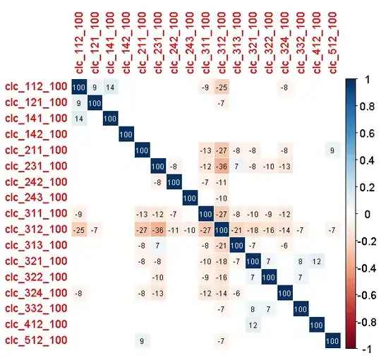
Could this be a problem with 1) fitting the model 2) model selection 3) predictions? This is not exactly collinearity (there is no correlation coefficient over 0.4 or under -0.4), but the variables are linearly dependent - the each one could be derived from all the others. If there is too much of a certain habitat, there cannot be a lot of other habitat types.

EDIT: The correlogram is here (the number is correlation coefficient multiplied by 100 and rounded. Only significant p < 0.05 coefficients are displayed).

enter image description here

EDIT 2: please do not assume that the variables are correlated. They are slightly in my case, but in general the variables can be linearly dependent but with no correlation! Look at this artificialy generated example:

set.seed(1063)
x <- rmultinom(17, rep(1000, 17), rep(1/17, 17))
envV <- x/1000

(If you have different RNG, please download the generated matrix: http://pastebin.com/sK55w3Y2)

Now the columns of envV are linearly dependent, as they sum up to 1 (see apply(envV, 2, sum)), but they are not correlated. See:

cor.mtest <- function(mat, conf.level = 0.95){
    mat <- as.matrix(mat)
    n <- ncol(mat)
    p.mat <- lowCI.mat <- uppCI.mat <- matrix(NA, n, n)
    diag(p.mat) <- 0
    diag(lowCI.mat) <- diag(uppCI.mat) <- 1
    for(i in 1:(n-1)){
        for(j in (i+1):n){
            tmp <- cor.test(mat[,i], mat[,j], conf.level = conf.level)
            p.mat[i,j] <- p.mat[j,i] <- tmp$p.value
   lowCI.mat[i,j] <- lowCI.mat[j,i] <- tmp$conf.int[1]
            uppCI.mat[i,j] <- uppCI.mat[j,i] <- tmp$conf.int[2]
        }
    }
    return(list(p.mat, lowCI.mat, uppCI.mat))
}

cor1 <- cor.mtest(envV)

number_of_correlated_variables <- sum(cor1[[1]] < 0.05 & !diag(nrow(cor1[[1]])))
number_of_correlated_variables  # reports 0

EDIT 3: It is interesting and strange that the matrix can be actually inverted: if I do solve(t(as.matrix(envV)) %*% as.matrix(envV)) both on my real predictors and the artificial generated ones in EDIT 2, the inverse matrix will get computed with no error or warning (both with solve and ginv()).

Also:

> is.singular.matrix(t(as.matrix(envV)) %*% as.matrix(envV))
[1] FALSE
Tomas
  • 5,735
  • 11
  • 52
  • 93
  • Related: http://stats.stackexchange.com/questions/54990/how-to-perform-multiple-regression-when-one-predictor-is-the-sum-of-two-other-pr You could adapt the answers from there. – kjetil b halvorsen Dec 30 '14 at 15:27
  • @kjetilbhalvorsen thanks. I think the important difference is that I have 17 variables instead of just 3, so as I mentined no correlation is actually strong (you can also see the correlogram) - the high number of variables make it kind of dilute, so the variables are less correlated but still linearly dependent. – Tomas Dec 30 '14 at 15:42
  • 17 instead of 3 isn't a meaningful difference. Regardless of the pairwise correlations, you have perfect multicollinearity. If all variables sum to 1, the value of the last variable can be determined perfectly by summing the 1st 16 and subtracting from $1$. – gung - Reinstate Monica Dec 30 '14 at 16:17
  • @gung, the definition of [perfect multicollinearity at wiki](http://en.wikipedia.org/wiki/Multicollinearity) says that the matrix is singular and cannot be inverted, which is not my case - see EDIT 3. How can I understand this? – Tomas Dec 30 '14 at 16:46
  • Curious: If your matrix is full rank, then the linear dependence is only approximate, not exact as you have told us. Tel us more about your actual variables, and how they were computed or measured. – kjetil b halvorsen Dec 30 '14 at 17:02
  • @kjetilbhalvorsen the linear dependence is *not* approximate - the variables sum exactly to 1. – Tomas Dec 30 '14 at 17:09
  • 3
    Curious: If so, then the matrix is **not** of full rank. If your software tells you it is, it is **wrong** and you should find better software! – kjetil b halvorsen Dec 30 '14 at 17:12
  • @kjetilbhalvorsen so are you suggesting that standard R functions like `solve`, `ginv` and `is.singular.matrix` (see EDIT 3) are *all* buggy? Not very likely, so please re-think your statement. You are welcome to look at the matrix I present in EDIT 2 and check it yourself! – Tomas Dec 30 '14 at 17:44
  • 1
    Curious: It is also the possibility you are misusing R. I guess you are confused. – kjetil b halvorsen Dec 30 '14 at 17:50
  • 1
    @Curious, you get "different" results with lm() and solve(), because you were supplyingh the design matrix without the intercept into solve(), while lm() adds it by default, as Khashaa noted – Aksakal Dec 30 '14 at 19:05
  • 1
    The sum sum to 1 thing isn't necessarily an issue. If this forum was open I could post a proof for linear independence in $\mathbf{X}$ (because you aren't including a constant). We do this kind of stuff in regression all the time with fixed effects. where we don't include an intercept and all the effects in the model, every row sums to one but the results of the regressions are still valid (and well published in academic research). – Zachary Blumenfeld Dec 30 '14 at 19:54
  • 3
    There are a couple of problems which I do find concerning in your simulation. 1) you have only 17 observations for 17 variables which essentially means you have zero degrees of freedom. 2) From the way you set up your simulation it looks like all the observations for each variable sum to 1, which is different from saying that the sum of all variables for each observation equals one. The latter is more pertinent to the discussion of this thread. Which one is it? – Zachary Blumenfeld Dec 30 '14 at 19:55
  • 1
    If the matrix isn't singular, I would guess that is due to numerical (eg, rounding) issues. The difference b/t the sum of a row & 1 might be something like 1 X 10^-30, which keeps it from being called singular when you ask, but you still have perfect multicollinearity in essence. – gung - Reinstate Monica Dec 30 '14 at 21:09

2 Answers2

4

The problem is that you have only 16 predictors, not 17. You can take any 16 variables and compute the remaining. This is the case of perfect milticollinearity. The solution is to simply regress on any subset of 16 variables.

The perfect multicollinearity (also rank deficiency) is the problem of identification in OLS. It's basically a technicality where you'd need to invert the design matrix $X'X$, and it's impossible when one of your variables is the linear combination of others.

Look up this wiki page for the definitions of the perfect multicollinearity condition: $\lambda_0 + \lambda_1 X_{1i} + \lambda_2 X_{2i} + \cdots + \lambda_k X_{ki} = 0$, which is what you have in your data with $k=17$, $\lambda_i=1, i\in [1,17]$ and $\lambda_0=-1$

UPDATE 3 Thanks to @Khashaa, he noticed that you did not use the intercept in your test, that's why it seems to pass. Here's the correct test code:

> x=runif(100*16)/17;
> x1=matrix(x,100,16)
> envV=cbind(x1,1-apply(x1,1,sum),rep(1,100))> apply(envV,1,sum)
  [1] 2 2 2 2 2 2 2 2 2 2 2 2 2 2 2 2 2 2 2 2 2 2 2 2 2 2 2 2 2 2 2 2 2 2 2 2 2
 [38] 2 2 2 2 2 2 2 2 2 2 2 2 2 2 2 2 2 2 2 2 2 2 2 2 2 2 2 2 2 2 2 2 2 2 2 2 2
 [75] 2 2 2 2 2 2 2 2 2 2 2 2 2 2 2 2 2 2 2 2 2 2 2 2 2 2
> hat=t(envV)%*%envV
> solve(hat)
Error in solve.default(hat) : 
  system is computationally singular: reciprocal condition number = 4.17876e-18

UPDATE 2 The reason why you don't see the correlations high is because you have a linear relationship with 17 variables, so pair-wise correlations don't have to be high. Consider this $x_{17}=1-\sum_{i=1}^{16}x_i, x_i\sim\mathcal{N}(0,1)$, if you look at the pair-wise correlations, you get $Corr[x_{17},x_i]=\frac{1}{\sqrt{16}}$, a relatively low number. So, in this case you're not going to notice multicollinearity by looking at pair-wise correlations.

Aksakal
  • 55,939
  • 5
  • 90
  • 176
  • I am afraid you are messing up linear dependence with correlation (collinearity). The fact that the variables sum up to 1 doesn't mean they are correlated - see the example I've added in the edit. – Tomas Dec 30 '14 at 16:16
  • @Curious, why don't you check the definition of [multicollinearity](http://en.wikipedia.org/wiki/Multicollinearity) and convince yourself that OP's data fits it? – Aksakal Dec 30 '14 at 16:19
  • 1) I am the OP :) 2) First sentence of the definition of Multicollinearity at wikipedia says "statistical phenomenon in which two or more predictor variables in a multiple regression model are **highly correlated**" - which they are not, see my EDIT 2 – Tomas Dec 30 '14 at 16:23
  • @Curious, read the rest of the sentence then "meaning that one can be linearly predicted from the others with a non-trivial degree of accuracy." – Aksakal Dec 30 '14 at 16:25
  • Thanks. 1) But why do they speak of correlation? The definition is clearly wrong 2) it is interesting that the matrix can actually be inverted, please see my EDIT 3. – Tomas Dec 30 '14 at 16:30
  • @Curious, it's not a wrong definition. There's a *perfect multicollinearity* and there's *multicollinearity*. In the former case you won't be able to invert the matrix, in the latter case technically you'll invert the matrix, but your model will have serious issues when it comes to interpretation of coefficients. The high level of correlation will be present in both cases. It may not be evident in pair-wise correlations. – Aksakal Dec 30 '14 at 16:33
  • 1) The definition *is* wrong because it messes up linear dependence and correlation - it implies that the variables must be correlated, which is not true, as I have shown. I would like to see a single consistent definition which we can use. 2) I don't know what you mean with "high level of correlation", there is none in my generated matrix in EDIT2. 3) The definition of "perfect multicollinearity" at wiki is that the matrix is singular and cannot be inverted, which doesn't apply to my case either. *So how can I see that the definitions you are proposing apply to my case?* – Tomas Dec 30 '14 at 16:43
  • 1
    @Curious I think @Aksakal assumed that intercept is included in your predictors. But I see no trace of it in `envV`. – Khashaa Dec 30 '14 at 17:08
  • See the result of `summary(lm(y~t(envV)))` for `y – Khashaa Dec 30 '14 at 17:13
  • @Curious, see my update on testing, I'll also comment on correlation. – Aksakal Dec 30 '14 at 17:31
  • @Khashaa Do you know why `lm` doesn't run, but `solve( t(envV) %*% envV ) %*% t(envV) %*% y` (i.e. $(X'X)^{-1}X'y$) runs fine? – Heisenberg Dec 30 '14 at 17:36
  • 2
    @Heisenberg `lm` automatically includes intercept thus creates multicollinearity. Sometimes people mistakenly include all the dummies in the regression, but fortunately `R` is smart enough to spot the error. – Khashaa Dec 30 '14 at 17:44
  • @Heisenberg, I think numerically the difference is that solve() uses LU decomposition, while lm.fit() uses QR decomposition. – Aksakal Dec 30 '14 at 17:49
  • @Khashaa, thanks for pointing out on the intercept – Aksakal Dec 30 '14 at 19:03
  • Curious, you misunderstand the Wikipedia quotation because you did not account for the second half of it: "...meaning that one can be linearly predicted from the others with a non-trivial degree of accuracy." That's quite different from saying that some coefficient of the correlation matrix is close to $\pm 1$! In Update 2, Aksakal gives an example of $17$ predictors where *by construction* one of them can be predicted with *perfect* accuracy from the other $16$, even though (with high probability) none of the correlation matrix coefficients will be large in size. – whuber Dec 30 '14 at 22:32
  • @Aksakal I don't think multicollinearity poses serious problems. If there is perfect multicollinearity, `R` will detect it. High correlations among covariates? "Do nothing" approach is better. – Khashaa Dec 31 '14 at 05:48
  • Completely irrelevant note on `R` programming: `apply` is just an euphemism for `for loop`. Vectorized version `rowSums(x1)` is infinitely faster than `apply(x1, 1, sum)`. – Khashaa Dec 31 '14 at 05:52
1

It could be an issue. Thinking of the design matrix, $X$ the last column could be expressed as $1 - $ sum of other columns. That means $X^TX$ would not be invertible.

Two options that might help, the first of which is probably going to be easier:

  • Drop a column. As its value is perfectly defined by the remaining data, you lose no information.
  • Use (Bayesian equivalent of) lasso regression, which will effectively choose one to drop for you.

Low entries in the correlogram are unlikely to signify we can relax. The proportions must be negatively related in some sense as for one to get larger, another must get smaller.

conjectures
  • 3,971
  • 19
  • 36
  • It is interesting and strange that the matrix can be actually inverted: if I do `solve(t(as.matrix(envV)) %*% as.matrix(envV))` both on my real predictors *and* the artificial generated ones in EDIT 2, the inverse matrix will get computed with no error or warning (both with `solve` and `ginv()`) – Tomas Dec 30 '14 at 16:28
  • @Curious, show us the code for artificially generated matrix test. – Aksakal Dec 30 '14 at 16:30
  • @Aksakal see EDIT 2. – Tomas Dec 30 '14 at 16:33
  • +1 thanks for the lasso tip! As for dropping the column, I don't think this is a good solution. If the habitat I drop is important for abundance of the species (response variable), I will loose its prediction power and significance of this coefficient (since all the other ones will have no important meaning for the species). – Tomas Dec 30 '14 at 16:59
  • 1
    @Curious, by dropping the column you will *NOT* lose anything. All the information from that column is contained in the remaining 16 columns. – Aksakal Dec 30 '14 at 18:37
  • @curious Have you tried inverting the design matrix with the intercept column attached? If you are using R and did not include -1 in the formulae this gets added with most functions. Try $X=$model.matrix(yourmodel) and try solve($X^T X$). – conjectures Dec 30 '14 at 21:54
  • The habitat you drop will be absorbed into the intercept, and the remaining coefficients should be contrasts from that baseline for each habitat. – conjectures Dec 30 '14 at 21:58
  • @conjectures Really? $n$ dimensional identity matrix $I_n$ satisfies the condition "the last column could be expressed as 1− sum of other columns", and if you know what I mean... – Khashaa Dec 31 '14 at 05:23
  • @Khashaa yes, if you have an intercept column in the design matrix. – conjectures Dec 31 '14 at 07:28