I kind of understand what "overfitting" means, but I need help as to how to come up with a real-world example that applies to overfitting.
Asked
Active
Viewed 4.1k times
115
-
12Perhaps you could explain what you 'kind of understand' about 'what overfitting means', so that people can address the parts you don't understand without having to guess what these might be? – goangit Dec 11 '14 at 09:45
-
http://www.tylervigen.com – shadowtalker Dec 11 '14 at 11:06
-
3@ssdecontrol Spurious correlation is not overfitting. In fact, spurious correlation need not involve an explicit model, and the implicit model is usually a straight line with two parameters. – Nick Cox Dec 11 '14 at 18:18
-
@user777 People look at it because it has a catchy title and it's on the "Hot questions" list. But then the question turns out to be very vague so people don't upvote. – David Richerby Dec 11 '14 at 19:22
-
@NickCox and who's to say you can't overfit a straight line? Sure it's not what you typically think of as overfitting, but if your model of the world is "these two things have a linear relationship" when they in fact do not, then I'd say your model is overfitted – shadowtalker Dec 11 '14 at 20:19
-
1@whuber: This would perhaps be more appropriate to discuss on meta, but I was surprised to see that you converted this post to community wiki. Doesn't it mean that the OP will not get reputation increase for future upvotes? To me it looks almost like a "punishment" for him; what was the reason for that? – amoeba Dec 11 '14 at 20:38
-
4@amoeba It's not punishment: this question as stated obviously has no one correct or canonical answer. In its original form as a non-CW question it was off-topic as a result--and should have rapidly been closed, BTW--but because there may be value in having some good examples created collectively by the community, conferring CW status *instead of closing it* seems to be a reasonable solution. – whuber Dec 11 '14 at 20:49
-
17So far **very few** of these answers (only two out of 11!) even attempt to address the question, which asks for a *real-world* example. That means not a simulation, not a theoretical example, not a cartoon, but a seriously applied model to actual data. Note, too, that the question explicitly tries to steer answers away from explanations of what overfitting is. – whuber Dec 11 '14 at 22:06
-
http://meta.stats.stackexchange.com/q/2301/2921. Let's take further discussion of this question to Meta. – D.W. Dec 12 '14 at 01:06
-
@ssdecontrol That defence seems tendentious to me. As spurious correlation usually arises from neglect of other variables, underfitting is arguably nearer the case. I'd still regard spurious correlation and overfitting as essentially unrelated. – Nick Cox Dec 14 '14 at 15:07
-
@NickCox I don't think it's tendentious at all and these correlations are most certainly not spurious because of omitted variable bias. I brought it up in Ten Fold and we can probably discuss it further there. – shadowtalker Dec 14 '14 at 19:04
-
@ssdecontrol Evidently I'm missing your point. Why not develop your argument as an answer? – Nick Cox Dec 15 '14 at 00:34
21 Answers
103
Here's a nice example of presidential election time series models from xkcd:

There have only been 56 presidential elections and 43 presidents. That is not a lot of data to learn from. When the predictor space expands to include things like having false teeth and the Scrabble point value of names, it's pretty easy for the model to go from fitting the generalizable features of the data (the signal) and to start matching the noise. When this happens, the fit on the historical data may improve, but the model will fail miserably when used to make inferences about future presidential elections.
dimitriy
- 31,081
- 5
- 63
- 138
-
15I think you should add something about sample bias to explain how this relates to overfitting. Just a cut&paste of the cartoon is missing the explanation. – Neil Slater Dec 11 '14 at 08:40
-
5A nice feature of this example is that it demonstrates the difference between overfitting and complexity. The rule "As goes California, so goes the nation" is simple, yet still overfit. – Tom Minka Dec 12 '14 at 20:42
-
2@TomMinka in fact overfitting can be caused by complexity (a model too complex to fit a too simple data, thus additional parameters will fit whatever comes at hand) or, as you pointed, by noisy features that gets more weights in the decision than pertinent features. And there are a lot of other possible sources of overfitting (intrinsic variance of the data or model, data not pertinent to represent the target goal, etc.). I think we ought to say that there are overfitting**s**, not just overfitting (which imply that there's just one cause, which often is not correct). – gaborous Dec 12 '14 at 22:09
87
My favorite was the Matlab example of US census population versus time:
- A linear model is pretty good
- A quadratic model is closer
- A quartic model predicts total annihilation starting next year
(At least I sincerely hope this is an example of overfitting)
http://www.mathworks.com/help/curvefit/examples/polynomial-curve-fitting.html#zmw57dd0e115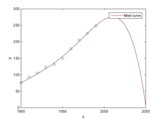
prototype
- 529
- 5
- 11
-
3Just to be clear exactly underneath the plot they do say : "The behavior of the sixth-degree polynomial fit beyond the data range makes it a poor choice for extrapolation and **you can reject this fit.**" – usεr11852 Apr 24 '15 at 05:59
-
1
51
The study of Chen et al. (2013) fits two cubics to a supposed discontinuity in life expectancy as a function of latitude.
Chen Y., Ebenstein, A., Greenstone, M., and Li, H. 2013. Evidence on the impact of sustained exposure to air pollution on life expectancy from China's Huai River policy. Proceedings of the National Academy of Sciences 110: 12936–12941. abstract
Despite its publication in an outstanding journal, etc., its tacit endorsement by distinguished people, etc., I would still present this as a prima facie example of over-fitting.
A tell-tale sign is the implausibility of cubics. Fitting a cubic implicitly assumes there is some reason why life expectancy would vary as a third-degree polynomial of the latitude where you live. That seems rather implausible: it is not easy to imagine a plausible physical mechanism that would cause such an effect.
See also the following blog post for a more detailed analysis of this paper: Evidence on the impact of sustained use of polynomial regression on causal inference (a claim that coal heating is reducing lifespan by 5 years for half a billion people).
Nick Cox
- 48,377
- 8
- 110
- 156
-
5+1 Andrew Gelman even wrote one or two blog posts about why it's implausible. Here's one: http://andrewgelman.com/2013/08/05/evidence-on-the-impact-of-sustained-use-of-polynomial-regression-on-causal-inference-a-claim-that-coal-heating-is-reducing-lifespan-by-5-years-for-half-a-billion-people/ – Sycorax Dec 11 '14 at 16:22
-
@user777 The Gelman blog is probably how I first heard of this. But I thought it most appropriate to give the reference, add the fluff of my personal comment, and let people judge for themselves. – Nick Cox Dec 11 '14 at 16:25
-
1I've cut an edit by @D.W. that introduced comments on life expectancy in different countries, which isn't what the paper is about at all. – Nick Cox Dec 12 '14 at 08:59
-
+1 - There are reasons for fitting the polynomial terms in RDD designs, but I have seen some pretty silly applications of it (one presentation I went to for "robustness" checks fit up to 9 polynomial terms - which if you've ever plotted a series of polynomial fits you will realize this is the opposite of robust!) – Andy W Dec 12 '14 at 14:22
-
2Another example I think is illustrative (although potentially more contrived than "real-world") are prediction competitions that feed-back intermediate results - like kaggle. Typically there are individuals who optimize results to the leaderboard, but they aren't the winners for the hold out sample. [Rob Hyndman](http://robjhyndman.com/hyndsight/prediction-competitions/) has some discussion of this. That takes a bit more in-depth perspective though than I think the OP wants here. – Andy W Dec 12 '14 at 14:24
-
2I was just about to post the Gelman & Imbens paper that came out of this: http://www.nber.org/papers/w20405 (gated, unfortunately) – shadowtalker Dec 12 '14 at 19:51
38
In a March 14, 2014 article in Science, David Lazer, Ryan Kennedy, Gary King, and Alessandro Vespignani identified problems in Google Flu Trends that they attribute to overfitting.
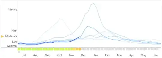
Here is how they tell the story, including their explanation of the nature of the overfitting and why it caused the algorithm to fail:
In February 2013, ... Nature reported that GFT was predicting more than double the proportion of doctor visits for influenza-like illness (ILI) than the Centers for Disease Control and Prevention (CDC) ... . This happened despite the fact that GFT was built to predict CDC reports. ...
Essentially, the methodology was to find the best matches among 50 million search terms to fit 1152 data points. The odds of finding search terms that match the propensity of the flu but are structurally unrelated, and so do not predict the future, were quite high. GFT developers, in fact, report weeding out seasonal search terms unrelated to the flu but strongly correlated to the CDC data, such as those regarding high school basketball. This should have been a warning that the big data were overfitting the small number of cases—a standard concern in data analysis. This ad hoc method of throwing out peculiar search terms failed when GFT completely missed the nonseasonal 2009 influenza A–H1N1 pandemic.
[Emphasis added.]
-
3Unfortunately this example has some problems. The paper suggests two rather different reasons why GFT was making bad predictions: overfitting and changes to the search engine. The authors admit that they are not in a position to determine which reason (if any) is correct, so it is essentially speculation. Furthermore, the paragraph about overfitting refers to the original version of the system, while the predictions in the graph were made with a modified system. – Tom Minka Dec 12 '14 at 19:36
-
1@Tom The article is not written as if the allegation of overfitting is speculation: the authors flatly assert that. I think it's a reasonable statement. They also address the reason why they have to be somewhat speculative: Google was not open or transparent about the algorithm. It seems to me immaterial for the present purpose whether the overfitting occurred only in one version or many, but as I recall the authors address this too and point out evidence of continued overfitting in the current algorithm. – whuber Dec 12 '14 at 19:46
-
2The article only says that overfitting is a standard concern in data analysis. It does not claim that overfitting was the reason. [Reference (2)](http://www.ploscompbiol.org/article/info%3Adoi%2F10.1371%2Fjournal.pcbi.1003256) goes into more detail, but again says that overfitting is only a "possible issue", with the statement "Because the search algorithm and resulting query terms that were used to define the original and updated GFT models remain undisclosed, it is difficult to identify the reasons for the suboptimal performance of the system and make recommendations for improvement." – Tom Minka Dec 12 '14 at 19:57
-
@Tom I will stand by the quotation given here, which is an accurate one, as adequate support for why the Google Flu model is worthy of consideration in the present context. – whuber Dec 12 '14 at 20:30
-
Interesting discussion. I'll add just that the graph might support the argument better if the lines were labeled. – rolando2 Dec 12 '14 at 21:27
-
@rolando2 I did not include a sort-of legend that appears in the original; it indicates that the truncated heavy blue line is for the 2014 season and the lighter blue lines are for "past years." It's actually a control you can use to limit the blue lines to a single year--you'll have to link to the site to use it. – whuber Dec 12 '14 at 22:00
35
I saw this image a few weeks ago and thought it was rather relevant to the question at hand.

Instead of linearly fitting the sequence, it was fitted with a quartic polynomial, which had perfect fit, but resulted in a clearly ridiculous answer.
March Ho
- 101
- 1
- 3
-
12This does not answer the question as asked, and might be better as a comment or not being posted at all. This does not provide a real-world example of overfitting (which is what the question asked for). It also does not explain how the example image is relevant to overfitting. Finally, it is very short. We prefer thorough, detailed answers that answer the question that was asked -- not just discussion related to the question. – D.W. Dec 12 '14 at 00:51
-
9In fact this is exactly a case of overfitting due to too-complex model, as you can construct an infinity of higher-order (non-linear) functions in order to generate an infinite number of different last terms of the sequence while still fitting the other (known) terms, by using a [Lagrange interpolation as explained here](http://math.stackexchange.com/a/341732/72736). – gaborous Dec 12 '14 at 22:24
-
2@user1121352 In the cartoon, the high-order polynomial **is** the true model, so it's not about over-fitting at all. An answer such as "9" (the next odd number) or "11" (the next odd prime) would actually be *under*-fitting because it uses a too-simple model to predict the next value. The cartoon actually illustrates the opposite case, that a more complex model could be true. – Sycorax Dec 13 '14 at 13:34
-
8The quartic polynomial (as interpreted by me) is intended to be a ridiculous solution, since the obvious answer that anyone will give before seeing the ridiculous solution would be 9 (or any other OEIS value). I assumed the "doge" format conveyed the sarcasm, but we clearly see Poe's Law at work here. – March Ho Dec 13 '14 at 14:01
-
2This is exactly the point I'm trying to make, though, which is that we don't know what the true function is. If you're conducting original analysis, you don't have a resource like the OEIS to appeal to for truth: that's what your model is attempting to establish. I appreciate that the cartoon is attempting sarcasm, but the cartoon's placement within this particular discussion exposes an important subtlety to the question about overfitting and statistical modelling generally. The intent of its original creator is irrelevant because you've recontextualized it here! – Sycorax Dec 13 '14 at 15:19
24
To me the best example is Ptolemaic system in astronomy. Ptolemy assumed that Earth is at the center of the universe, and created a sophisticated system of nested circular orbits, which would explain movements of object on the sky pretty well. Astronomers had to keep adding circles to explain deviation, until one day it got so convoluted that folks started doubting it. That's when Copernicus came up with a more realistic model.
This is the best example of overfitting to me. You can't overfit data generating process (DGP) to the data. You can only overfit misspecified model. Almost all our models in social sciences are misspecified, so the key is to remember this, and keep them parsimonious. Not to try to catch every aspect of the data set, but try to capture the essential features through simplification.
Aksakal
- 55,939
- 5
- 90
- 176
-
15This does not appear to be an example of overfitting. There's nothing wrong with the Ptolemaic system as a predictive model: it is complicated only because the coordinate system is geocentric rather than originating with the galactic center of mass. The problem, therefore, is that an accurate, legitimate fit was made with an overly complicated model. (Ellipses are much simpler than epicycles.) It's a true challenge to find parsimonious nonlinear models! – whuber Dec 11 '14 at 18:03
-
1You'll end up with a lot of circles to model Jupiter's moons' orbits in Ptolemaic system. – Aksakal Dec 11 '14 at 18:06
-
19That's right--but on the face of it, that's not necessarily overfitting. The acid test lies in the predictions of future values, which in that system worked well enough to stand for 1400 years. Data are *overfit* not when the model is very complicated, but when it is so *flexible* that by capturing extraneous detail it produces much more inaccurate predictions than would be expected from an analysis of the model's residuals on its training data. – whuber Dec 11 '14 at 18:34
-
1"You can't overfit data generating process (DGP) to the data. You can only overfit misspecified model." is rather unclear. It's incorrect if it means that correctly specifying the model to reflect the data-generating process (when this is feasible) is any guarantee against over-fitting. – Scortchi - Reinstate Monica Dec 12 '14 at 13:26
-
@Scortchi, I don't think you can overfit correctly specified model. The problem's that maybe physics and engineering are the only areas where we ever correctly specify the models. In social sciences there's not a chance. – Aksakal Dec 12 '14 at 13:54
-
2Aksakal: You certainly can. Consider @arnaud's example, & suppose the data-generating process were known to be $\operatorname{E}Y=\sum_{k=0}^9 \beta_k x^i$. Would learning that lead you to *fit* that model to those ten data points in the expectation of better predictions on new data than the simple linear model? – Scortchi - Reinstate Monica Dec 12 '14 at 14:46
-
Sample size for 10 parameters is not a regression at all. It's a linear equation system. – Aksakal Dec 12 '14 at 14:48
-
Don't know what you mean by that. BTW there was a typo in my comment - I meant of course $\operatorname{E}Y=\sum_{k=0}^9 \beta_k x_k$. – Scortchi - Reinstate Monica Dec 12 '14 at 15:00
-
You said there's 10 data points. You have 11 parameters in the model. This is not a regression model at all. In fact, this is not a linear system either, you have one extra parameter. This can't be solved at all. This is not a good example for your argument. – Aksakal Dec 12 '14 at 15:04
-
2@Aksakal: 10 parameters: $\operatorname{E}Y=\sum_{k=0}^9 \beta_k x^k$ (typed correctly now!). Of course the error can't be estimated, or assume it known. If it's bothering you, consider an eighth-order polynomial in $x$; the point's the same. – Scortchi - Reinstate Monica Dec 12 '14 at 15:15
-
1There is another reason why it's very bad example. Astronomers did not start with many circles and find the model to fit well and they did not throw many different models at the data and select circles because they worked well on past data. They had to use circles for aesthetic, religious and practical reasons and kept adding some to improve predictions. That process is less than ideal but it feels like the opposite of overfitting to me. – Gala Dec 13 '14 at 08:14
-
1@aksakal If you look at [my answer](http://stats.stackexchange.com/a/128719/22228) you'll see R code for simulation that allows you to experiment with overfitting. Perform the modifications described in my final bullet point. You'll discover that by fitting the correct model to small n you get worse predictive performance *even on the holdout set* than using a simplified model. Hence, overfit. – Silverfish Dec 13 '14 at 22:18
-
1@aksakal Roughly, the correct model may include parameters hard to estimate from small n; then the model has too many df so too much flexibility and will use this to "fit the noise" rather than the signal (so will generalise poorly when making predictions on a holdout set). But with larger n it's easier to detect the underlying signal, reasonable parameter estimates can be made, and the true model can outperform predictions made by a simpler model. Overfitting can depend on sample size not just model correctness/complexity, which is something this answer doesn't make clear. – Silverfish Dec 13 '14 at 22:27
-
@Silverfish, I see that you're modeling GDP. Nobody models it like this, trust me. Your example is misleading as you're trying to fit clearly wrong model to demonstrate over-fitting, while your problem there is simply misspecification. Small$n$ is an entirely different issue. Tjere's no point is *statistics" when the number of observations is barely larger than the number of parameters. It's like having one observation and trying to apply statistics to it. – Aksakal Dec 13 '14 at 22:28
-
1@aksakal The simulation at the bottom is not related to the GDP graph at the top, in fact I didn't give any contextual meaning to it. Perhaps I should have submitted as two separate answers. I'm confused by your statement - there are many techniques for modelling data with "small n, large p". Sample size *is* relevant to overfitting, and a correct model can be overfit if it is too complex for the available data. Despite omitted variable bias, a more parsimonious model can have better predictive performance in this situation. – Silverfish Dec 13 '14 at 22:45
-
1@aksakal might the "misleading" example convince you? Suppose data like that (doesn't have to be GDP) didn't have a completely linear relationship in the population - unless there were a physical law at work that'd hardly be surprising. Polynomial fit for a curvilinear relationship is reasonable. Imagine it were only *slightly* curved, so true coefficient of $x^2$ is 0.00000001 and so on. Barely different from 0. Now the polynomial fit *isn't* "misspecified" but such a model still has too much flexibility for the data, will overfit, and prediction will be be just as poor as illustrated. – Silverfish Dec 14 '14 at 00:03
-
@Silverfish, I apologize, shouldn't have used "misleading". If you know the underlying law (equation), then you should use it. If there's not enough data, get it. In physical sciences that's how it works. In social sciences we never really know the *true* equation, and we're usually confined with observational data, i.e. we can't get more data. So, we have to differentiate these situations. It doesn't make a sense to talk about *true* models in social sciences at all. – Aksakal Dec 14 '14 at 03:46
-
1Even if there is a correct model, given limited data, a more parsimonious model that extracts key features can have better predictive performance. This is what scortchi said re arnaud's example - if the DGP were an 8th power polynomial, that would still be overfit. A linear model would make better predictions from the data than the correct model. – Silverfish Dec 14 '14 at 08:37
-
@Aksaksal: I love your answer. I independently just thought of the Ptolemaic system as a good example of overfitting. Although it is not so straightforward to explain why, the Ptolemaic system screams of "overfitting" and one of the best examples at that. – ColorStatistics Apr 28 '20 at 04:10
-
@whuber: You're thinking of overfitting only in the predictive sense. There is also overfitting in a causal sense, and in fact that is likely to have been the context here. They were looking to understand what was causing the apparent motions in the sky and not merely to predict where a planet will be in a week. If we think causally (what is causing the paths of motion of different planets, stars), the overfitting becomes apparent. – ColorStatistics Apr 28 '20 at 04:19
-
A causal model needs to be formulated before seeing the data and not data mined (in the economists' sense of the word)/overfit to the data. What Ptolemy did was to formulate his causal model so as to fit the data at hand as well as possible. His model got the causality totally wrong (certainly the retrograde motion is not due to epicycles, equants, etc.) because of the overfitting. – ColorStatistics Apr 28 '20 at 04:22
-
@ColorStatistics I think Ptolemy had a few successful predictions. I’m not sure if those were by chance or because his system worked like a non orthogonal function expansion. – Aksakal Apr 28 '20 at 13:30
-
I am not sure what you mean by "non-orthogonal function expansion". Based on what I read, I agree that it looks like his model did a pretty good job at predicting, but it was certainly the wrong/completely overfit causal mechanism, much like whether people carry umbrellas in the morning will likely be helpful in predicting whether it will ran that day but the carrying of umbrellas certainly does not cause the rain. The context of his work was certainly causal and not prediction. They were trying to figure out the structure of the solar system, and not merely predict movements in the sky. – ColorStatistics Apr 28 '20 at 14:33
-
1@ColorStatistics, I wouldn't say Ptolemy's system was so good at predicting out of sample, but they were good at presenting selective evidence. Since, it's been declared God;s system, they had to hide contradictions for centuries. By non-orthogonal, I mean that any function can be presented as sum $f(x)=\sum_i a_i g_i(x)$ where $g_i(x)$ a set of other functions. This works best when you plug these into the equations of the system, and when $g_i$ happen to be eigen functions of it. Then you get the orthogonal expansion such as Fourier or Bessel. – Aksakal Apr 28 '20 at 14:41
-
@ColorStatistics, since Ptolemy didn't have a "true" system of equations, his circles were not the correct orthogonal system of eigen functions for celestial movements, thus his expansion didn't work very well. But conceptually to me he was doing the right thing by factoring the complex movement into simple movements, if only he could choose the correct system of simple movements, and if only the true system even allowed for such a system to exist – Aksakal Apr 28 '20 at 14:44
-
23
Let's say you have 100 dots on a graph.
You could say: hmm, I want to predict the next one.
- with a line
- with a 2nd order polynomial
- with a 3rd order polynomial
- ...
- with a 100th order polynomial
Here you can see a simplified illustration for this example:
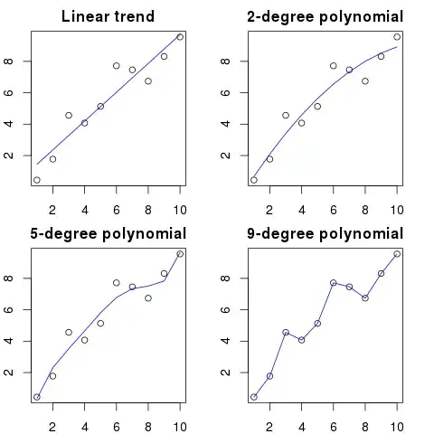
The higher the polynomial order, the better it will fit the existing dots.
However, the high order polynomials, despite looking like to be better models for the dots, are actually overfitting them. It models the noise rather than the true data distribution.
As a consequence, if you add a new dot to the graph with your perfectly fitting curve, it'll probably be further away from the curve than if you used a simpler low order polynomial.
-
"As a consequence, if you add a new dot to the graph with your perfectly fitting curve, it'll probably be further away from the curve than if you used a simpler low order polynomial" - moreover, this is still true even if the data-generating process for the new dot (ie the relationship in the population) was actually a high power polynomial like the one you (over)fitted. – Silverfish Dec 14 '14 at 08:42
-
20The pictures here are actually incorrect - for example, the 9-degree polynomial has only been plotted as a piecewise linear function, but I suspect in reality it should swing wildly up & down in the ranges between the points. You should see this effect in the 5-degree polynomial too. – Ken Williams Dec 16 '14 at 16:46
20
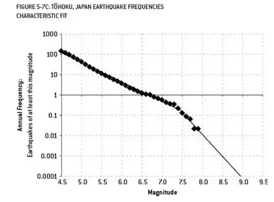
The analysis that may have contributed to the Fukushima disaster is an example of overfitting. There is a well known relationship in Earth Science that describes the probability of earthquakes of a certain size, given the observed frequency of "lesser" earthquakes. This is known as the Gutenberg-Richter relationship, and it provides a straight-line log fit over many decades. Analysis of the earthquake risk in the vicinity of the reactor (this diagram from Nate Silver's excellent book "The Signal and the Noise") show a "kink" in the data. Ignoring the kink leads to an estimate of the annualized risk of a magnitude 9 earthquake as about 1 in 300 - definitely something to prepare for. However, overfitting a dual slope line (as was apparently done during the initial risk assessment for the reactors) reduces the risk prediction to about 1 in 13,000 years. One could not fault the engineers for not designing the reactors to withstand such an unlikely event - but one should definitely fault the statisticians who overfitted (and then extrapolated) the data...
Floris
- 503
- 3
- 7
-
Is it conclusive the dual slope model was overfit? The kink is prominent; I'd guess if each line segment was estimated from, say, 3 points each, you'd get better predictions on the hold-out than by estimating a single line. (Of course the subsequent observation of a "1 in 13,000 yr" event argues against it! But that's hard to interpret as we wouldn't be re-examining this model if that hadn't happened.) If there were physical reasons to ignore the perceived kink then the case this was overfit is stronger - I don't know how well such data usually matches the ideal Gutenberg-Richter relationship. – Silverfish Dec 16 '14 at 02:16
-
This does very graphically illustrate the perils of extrapolation, and the need for a loss function that takes into account the severity of consequences of an error... – Silverfish Dec 16 '14 at 02:20
-
3The problem really is that very little data is used for some of the last points - so they have a great deal of uncertainty in them. Looking closely at the data, you can see there was a single 7.9 event, then several 7.7s. Little is known about quakes greater than 8.0 as they are infrequent - but when you observe a 9.0 quake (the Tohoku quake that caused the Tsunami) you can draw your own conclusion. The straight line may be conservative - but when it comes to nuclear safety, conservative is good. – Floris Dec 16 '14 at 03:13
-
I agree, here conservative is good. What got me thinking was this: imagine the data looked essentially the same, except that the kink went the other way (shallowed out). Then if the analysts fitted a straight line model, it would underplay risks of high-magnitude quake compared to a model (two slope or otherwise) that accounted for the kink. Would we suspect the analysts of *underfitting*? I think if I lived near the nuclear plant, I might! – Silverfish Dec 16 '14 at 19:08
-
1@Floris Good point. It would have been better if they had used a box-plot that showed not only the observed frequencies but also confidence intervals for those frequencies. Then one would probably get very narrow boxes to the left in the diagram and very wide boxes to the right. (Such confidence intervals can be calculated assuming that each frequency follows a Poisson distribution.) – user763305 Dec 17 '14 at 13:01
-
3@user763305 - yes, I'm pretty sure that adding confidence intervals would show that a straight line is not inconsistent with the data (or in other words, that you can't reject the null hypothesis that the data follow a straight line). – Floris Dec 17 '14 at 14:13
-
19
"Agh! Pat is leaving the company. How are we ever going to find a replacement?"
Job Posting:
Wanted: Electrical Engineer. 42 year old androgynous person with degrees in Electrical Engineering, mathematics, and animal husbandry. Must be 68 inches tall with brown hair, a mole over the left eye, and prone to long winded diatribes against geese and misuse of the word 'counsel'.
In a mathematical sense, overfitting often refers to making a model with more parameters than are necessary, resulting in a better fit for a specific data set, but without capturing relevant details necessary to fit other data sets from the class of interest.
In the above example, the poster is unable to differentiate the relevant from irrelevant characteristics. The resulting qualifications are likely only met by the one person that they already know is right for the job (but no longer wants it).
Mark Borgerding
- 129
- 5
-
8While entertaining, this answer does not provide insight into what overfitting means in a statistical sense. Perhaps you could expand your answer to clarify the relationship between these very particular attributes and statistical modeling. – Sycorax Dec 11 '14 at 14:52
-
+1 Mark. I agree with @user777 only to a small extent. Maybe a sentence will bring the concise example home. But adding too much will take away from the simplicity. – ndoogan Dec 11 '14 at 14:58
-
I think this is a great answer - it exhibits the very common type of overfitting that essentially memorizes the training data, especially the common case when the amount of training data is insufficient to saturate the expressive power of the model. – Ken Williams Dec 16 '14 at 16:49
16
This one is made-up, but I hope it will illustrate the case.
Example 1
First, let's make up some random data. Here you have $k=100$ variables, each drawn from a standard normal distribution, with $n=100$ cases:
set.seed(123)
k <- 100
data <- replicate(k, rnorm(100))
colnames(data) <- make.names(1:k)
data <- as.data.frame(data)
Now, let's fit a linear regression to it:
fit <- lm(X1 ~ ., data=data)
And here is a summary for first ten predictors:
> summary(fit)

Call:
lm(formula = X1 ~ ., data = data)

Residuals:
ALL 100 residuals are 0: no residual degrees of freedom!

Coefficients:
              Estimate Std. Error t value Pr(>|t|)
(Intercept) -1.502e-01         NA      NA       NA
X2           3.153e-02         NA      NA       NA
X3          -6.200e-01         NA      NA       NA
X4           7.087e-01         NA      NA       NA
X5           4.392e-01         NA      NA       NA
X6           2.979e-01         NA      NA       NA
X7          -9.092e-02         NA      NA       NA
X8          -5.783e-01         NA      NA       NA
X9           5.965e-01         NA      NA       NA
X10         -8.289e-01         NA      NA       NA
...
Residual standard error: NaN on 0 degrees of freedom
Multiple R-squared:      1, Adjusted R-squared:    NaN
F-statistic:   NaN on 99 and 0 DF,  p-value: NA
results look pretty weird, but let's plot it.
That is great, fitted values perfectly fit the $X_1$ values. Error variance is literally zero. But, let it not convince us, let's check what is the sum of absolute differences between $X_1$ and fitted values:
> sum(abs(data$X1-fitted(fit)))
[1] 0
It is zero, so the plots were not lying to us: the model fits perfectly. And how precise is it in classification?
> sum(data$X1==fitted(fit))
[1] 100
We get 100 out of 100 fitted values that are identical to $X_1$. And we got this with totally random numbers fitted to other totally random numbers.
Example 2
One more example. Lets make up some more data:
data2 <- cbind(1:10, diag(10))
colnames(data2) <- make.names(1:11)
data2 <- as.data.frame(data2)
so it looks like this:
   X1 X2 X3 X4 X5 X6 X7 X8 X9 X10 X11
1   1  1  0  0  0  0  0  0  0   0   0
2   2  0  1  0  0  0  0  0  0   0   0
3   3  0  0  1  0  0  0  0  0   0   0
4   4  0  0  0  1  0  0  0  0   0   0
5   5  0  0  0  0  1  0  0  0   0   0
6   6  0  0  0  0  0  1  0  0   0   0
7   7  0  0  0  0  0  0  1  0   0   0
8   8  0  0  0  0  0  0  0  1   0   0
9   9  0  0  0  0  0  0  0  0   1   0
10 10  0  0  0  0  0  0  0  0   0   1
and now lets fit a linear regression to this:
fit2 <- lm(X1~., data2)
so we get following estimates:
> summary(fit2)

Call:
lm(formula = X1 ~ ., data = data2)

Residuals:
ALL 10 residuals are 0: no residual degrees of freedom!

Coefficients: (1 not defined because of singularities)
            Estimate Std. Error t value Pr(>|t|)
(Intercept)       10         NA      NA       NA
X2                -9         NA      NA       NA
X3                -8         NA      NA       NA
X4                -7         NA      NA       NA
X5                -6         NA      NA       NA
X6                -5         NA      NA       NA
X7                -4         NA      NA       NA
X8                -3         NA      NA       NA
X9                -2         NA      NA       NA
X10               -1         NA      NA       NA
X11               NA         NA      NA       NA

Residual standard error: NaN on 0 degrees of freedom
Multiple R-squared:      1, Adjusted R-squared:    NaN
F-statistic:   NaN on 9 and 0 DF,  p-value: NA
as you can see, we have $R^2 = 1$, i.e. "100% variance explained". Linear regression didn't even need to use 10th predictor. From this regression we see, that $X_1$ can be predicted using function:
$$X_1 = 10 + X_2 \times -9 + X_3 \times -8 + X_4 \times -7 + X_5 \times -6 + X_6 \times -5 + X_7 \times -4 + X_8 \times -3 + X_9 \times -2$$
so $X_1 = 1$ is:
$$10 + 1 \times -9 + 0 \times -8 + 0 \times -7 + 0 \times -6 + 0 \times -5 + 0 \times -4 + 0 \times -3 + 0 \times -2$$
It is pretty self-explanatory. You can think of Example 1 as similar to Example 2 but with some "noise" added. If you have big enough data and use it for "predicting" something then sometimes a single "feature" may convince you that you have a "pattern" that describes your dependent variable well, while it could be just a coincidence. In Example 2 nothing is really predicted, but exactly the same has happened in Example 1 just the values of the variables were different.
Real life examples
The real life example for this is predicting terrorist attacks on 11 September 2001 by watching "patterns" in numbers randomly drawn by computer pseudorandom number generators by Global Consciousness Project or "secret messages" in "Moby Dick" that reveal facts about assassinations of famous people (inspired by similar findings in Bible).
Conclusion
If you look hard enough, you'll find "patterns" for anything. However, those patterns won't let you learn anything about the universe and won't help you reach any general conclusions. They will fit perfectly to your data, but would be useless since they won't fit anything else then the data itself. They won't let you make any reasonable out-of-sample predictions, because what they would do, is they would rather imitate than describe the data.
Tim
- 108,699
- 20
- 212
- 390
-
5I'd suggest putting the real-life examples at the _top_ of this answer. That's the part that's actually relevant to the question -- the rest is gravy. – shadowtalker Dec 12 '14 at 19:54
8
A common problem that results in overfitting in real life is that in addition to terms for a correctly specified model, we may have have added something extraneous: irrelevant powers (or other transformations) of the correct terms, irrelevant variables, or irrelevant interactions.
This happens in multiple regression if you add a variable that should not appear in the correctly specified model but do not want to drop it because you are afraid of inducing omitted variable bias. Of course, you have no way of knowing you have wrongly included it, since you can't see the whole population, only your sample, so can't know for sure what the correct specification is. (As @Scortchi points out in the comments, there may be no such thing as a the "correct" model specification - in that sense, the aim of modelling is finding a "good enough" specification; to avoid overfitting involves avoiding a model complexity greater than can be sustained from the available data.) If you want a real-world example of overfitting, this happens every time you throw all the potential predictors into a regression model, should any of them in fact have no relationship with the response once the effects of others are partialled out.
With this type of overfitting, the good news is that inclusion of these irrelevant terms does not introduce bias of your estimators, and in very large samples the coefficients of the irrelevant terms should be close to zero. But there is also bad news: because the limited information from your sample is now being used to estimate more parameters, it can only do so with less precision - so the standard errors on the genuinely relevant terms increase. That also means they're likely to be further from the true values than estimates from a correctly specified regression, which in turn means that if given new values of your explanatory variables, the predictions from the overfitted model will tend to be less accurate than for the correctly specified model.
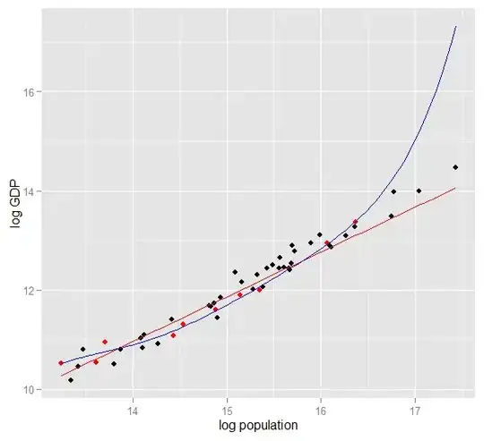
Here is a plot of log GDP against log population for 50 US states in 2010. A random sample of 10 states was selected (highlighted in red) and for that sample we fit a simple linear model and a polynomial of degree 5. For the sample points, the polynomial has extra degrees of freedom that let it "wriggle" closer to the observed data than the straight line can. But the 50 states as a whole obey a nearly linear relationship, so the predictive performance of the polynomial model on the 40 out-of-sample points is very poor compared to the less complex model, particularly when extrapolating. The polynomial was effectively fitting some of the random structure (noise) of the sample, which did not generalise to the wider population. It was particularly poor at extrapolating beyond the observed range of the sample. (Code plus data for this plot is at the bottom of this revision of this answer.)
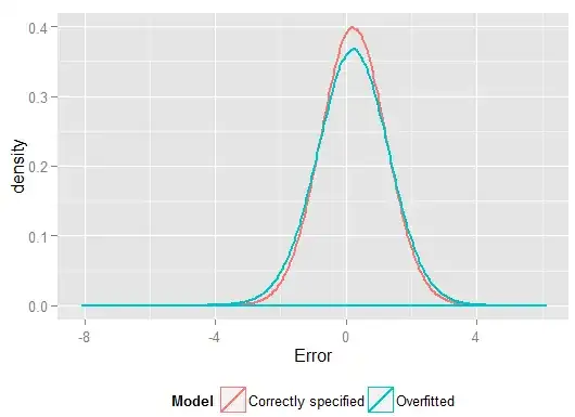
Similar issues affect regression against multiple predictors. To look at some actual data, it's easier with simulation rather than real-world samples since this way you control the data-generating process (effectively, you get to see the "population" and the true relationship). In this R code, the true model is $y_i = 2x_{1,i} + 5 + \epsilon_i$ but data is also provided on irrelevant variables $x_2$ and $x_3$. I have designed the simulation so that the the predictor variables are correlated, which would be a common occurrence in real-life data. We fit models which are correctly specified and overfitted (includes the irrelevant predictors and their interactions) on one portion of the generated data, then compare predictive performance on a holdout set. The multicollinearity of the predictors makes life even harder for the overfitted model, since it becomes harder for it to pick apart the effects of $x_1$, $x_2$ and $x_3$, but note that this does not bias any of the coefficient estimators.
require(MASS) #for multivariate normal simulation
nsample <- 25   #sample to regress
nholdout <- 1e6  #to check model predictions
Sigma <- matrix(c(1, 0.5, 0.4, 0.5, 1, 0.3, 0.4, 0.3, 1), nrow=3)
df <- as.data.frame(mvrnorm(n=(nsample+nholdout), mu=c(5,5,5), Sigma=Sigma))
colnames(df) <- c("x1", "x2", "x3")
df$y <- 5 + 2 * df$x1 + rnorm(n=nrow(df)) #y = 5 + *x1 + e

holdout.df <- df[1:nholdout,]
regress.df <- df[(nholdout+1):(nholdout+nsample),]

overfit.lm <- lm(y ~ x1*x2*x3, regress.df)
correctspec.lm <- lm(y ~ x1, regress.df)
summary(overfit.lm)
summary(correctspec.lm)

holdout.df$overfitPred <- predict.lm(overfit.lm, newdata=holdout.df)
holdout.df$correctSpecPred <- predict.lm(correctspec.lm, newdata=holdout.df)
with(holdout.df, sum((y - overfitPred)^2)) #SSE
with(holdout.df, sum((y - correctSpecPred)^2))

require(ggplot2)
errors.df <- data.frame(
    Model = rep(c("Overfitted", "Correctly specified"), each=nholdout),
    Error = with(holdout.df, c(y - overfitPred, y - correctSpecPred)))
ggplot(errors.df, aes(x=Error, color=Model)) + geom_density(size=1) +
    theme(legend.position="bottom")
Here are my results from one run, but it's best to run the simulation several times to see the effect of different generated samples.
>     summary(overfit.lm)

Call:
lm(formula = y ~ x1 * x2 * x3, data = regress.df)

Residuals:
     Min       1Q   Median       3Q      Max
-2.22294 -0.63142 -0.09491  0.51983  2.24193

Coefficients:
            Estimate Std. Error t value Pr(>|t|)
(Intercept) 18.85992   65.00775   0.290    0.775
x1          -2.40912   11.90433  -0.202    0.842
x2          -2.13777   12.48892  -0.171    0.866
x3          -1.13941   12.94670  -0.088    0.931
x1:x2        0.78280    2.25867   0.347    0.733
x1:x3        0.53616    2.30834   0.232    0.819
x2:x3        0.08019    2.49028   0.032    0.975
x1:x2:x3    -0.08584    0.43891  -0.196    0.847

Residual standard error: 1.101 on 17 degrees of freedom
Multiple R-squared: 0.8297,     Adjusted R-squared: 0.7596
F-statistic: 11.84 on 7 and 17 DF,  p-value: 1.942e-05
These coefficient estimates for the overfitted model are terrible - should be about 5 for the intercept, 2 for $x_1$ and 0 for the rest. But the standard errors are also large. The correct values for those parameters do lie well within the 95% confidence intervals in each case. The $R^2$ is 0.8297 which suggests a reasonable fit.
>     summary(correctspec.lm)

Call:
lm(formula = y ~ x1, data = regress.df)

Residuals:
    Min      1Q  Median      3Q     Max
-2.4951 -0.4112 -0.2000  0.7876  2.1706

Coefficients:
            Estimate Std. Error t value Pr(>|t|)
(Intercept)   4.7844     1.1272   4.244 0.000306 ***
x1            1.9974     0.2108   9.476 2.09e-09 ***
---
Signif. codes:  0 ‘***’ 0.001 ‘**’ 0.01 ‘*’ 0.05 ‘.’ 0.1 ‘ ’ 1

Residual standard error: 1.036 on 23 degrees of freedom
Multiple R-squared: 0.7961,     Adjusted R-squared: 0.7872
F-statistic:  89.8 on 1 and 23 DF,  p-value: 2.089e-09
The coefficient estimates are much better for the correctly specified model. But note that the $R^2$ is lower, at 0.7961, as the less complex model has less flexibility in fitting the observed responses. $R^2$ is more dangerous than useful in this case!
>     with(holdout.df, sum((y - overfitPred)^2)) #SSE
[1] 1271557
>     with(holdout.df, sum((y - correctSpecPred)^2))
[1] 1052217
The higher $R^2$ on the sample we regressed on showed how the overfitted model produced predictions, $\hat{y}$, that were closer to the observed $y$ than the correctly specified model could. But that's because it was overfitting to that data (and had more degrees of freedom to do so than the correctly specified model did, so could produce a "better" fit). Look at the Sum of Squared Errors for the predictions on the holdout set, which we didn't use to estimate the regression coefficients from, and we can see how much worse the overfitted model has performed. In reality the correctly specified model is the one which makes the best predictions. We shouldn't base our assessment of the predictive performance on the results from the set of data we used to estimate the models. Here's a density plot of the errors, with the correct model specification producing more errors close to 0:
The simulation clearly represents many relevant real-life situations (just imagine any real-life response which depends on a single predictor, and imagine including extraneous "predictors" into the model) but has the benefit that you can play with the data-generating process, the sample sizes, the nature of the overfitted model and so on. This is the best way you can examine the effects of overfitting since for observed data you don't generally have access to the DGP, and it's still "real" data in the sense that you can examine and use it. Here are some worthwhile ideas that you should experiment with:
- Run the simulation several times and see how the results differ. You will find more variability using small sample sizes than large ones.
- Try changing the sample sizes. If increased to, say,
n <- 1e6, then the overfitted model eventually estimates reasonable coefficients (about 5 for intercept, about 2 for $x_1$, about 0 for everything else) and its predictive performance as measured by SSE doesn't trail the correctly specified model so badly. Conversely, try fitting on a very small sample (bear in mind you need to leave enough degrees of freedom to estimate all the coefficients) and you will see that the overfitted model has appalling performance both for estimating coefficients and predicting for new data. - Try reducing the correlation between the predictor variables by playing with the off-diagonal elements of the variance-covariance matrix
Sigma. Just remember to keep it positive semi-definite (which includes being symmetric). You should find if you reduce the multicollinearity, the overfitted model doesn't perform quite so badly. But bear in mind that correlated predictors do occur in real life. - Try experimenting with the specification of the overfitted model. What if you include polynomial terms?
- What if you simulate data for a different region of predictors, rather than having their mean all around 5? If the correct data generating process for $y$ is still
df$y <- 5 + 2*df$x1 + rnorm(n=nrow(df)), see how well the models fitted to the original data can predict that $y$. Depending on how you generate the $x_i$ values, you may find that extrapolation with the overfitted model produces predictions far worse than the correctly specified model. - What if you change the data generating process so that $y$ now depends, weakly, on $x_2$, $x3$ and perhaps the interactions as well? This may be a more realistic scenario that depending on $x_1$ alone. If you use e.g.
df$y <- 5 + 2 * df$x1 + 0.1*df$x2 + 0.1*df$x3 + rnorm(n=nrow(df))then $x_2$ and $x_3$ are "almost irrelevant", but not quite. (Note that I drew all the $x$ variables from the same range, so it does make sense to compare their coefficients like that.) Then the simple model involving only $x_1$ suffers omitted variable bias, though since $x_2$ and $x_3$ are not particularly important, this is not too severe. On a small sample, e.g.nsample <- 25, the full model is still overfitted, despite being a better representation of the underlying population, and on repeated simulations its predictive performance on the holdout set is still consistently worse. With such limited data, it's more important to get a good estimate for the coefficient of $x_1$ than to expend information on the luxury of estimating the less important coefficients. With the effects of $x_2$ and $x_3$ being so hard to discern in a small sample, the full model is effectively using the flexibility from its extra degrees of freedom to "fit the noise" and this generalises poorly. But withnsample <- 1e6, it can estimate the weaker effects pretty well, and simulations show the complex model has predictive power that outperforms the simple one. This shows how "overfitting" is an issue of both model complexity and the available data.
Silverfish
- 20,678
- 23
- 92
- 180
-
1(-1) It's rather important to understand that over-fitting doesn't solely result from the inclusion of "irrelevant" or "extraneous" terms that wouldn't appear in a correctly specified model. Indeed it might be argued that in many applications the idea of a simple *true* model doesn't make much sense & the challenge of predictive modelling is to build a model whose complexity is proportioned to the amount of available data. – Scortchi - Reinstate Monica Dec 12 '14 at 11:34
-
Extend your example by giving *small* non-zero coefficients to $x_2$, $x_3$, & the interactions: fitting the full (correctly specified) model will result in a similar degree of over-fitting for this sample size, but lead to an improvement in predictive performance on larger samples. (BTW you may as well use a larger hold-out in a simulation as 50 is going to give very variable results.) – Scortchi - Reinstate Monica Dec 12 '14 at 11:35
-
@Scortchi Thanks, I agree. I intended this answer as a *basic example* of overfitting in real-life, and one which most readers are likely to have come across when they first looked at model selection for multiple regression. (A common exercise in classes seems to be the extreme example of "improving" $R^2$ by regressing against more noise variables.) I didn't intend it to represent overfitting in general but I have tried to improve the wording to reflect that! Your other suggestions are helpful - they show the transition from my extreme case to the more general case. I've tried to incorporate. – Silverfish Dec 12 '14 at 22:08
-
1I'll send your picture to my Congressman in support of immigration reform – prototype Dec 12 '14 at 22:22
-
1(+1) I think the edits improve the explanation of over-fitting without sacrificing understandability. – Scortchi - Reinstate Monica Dec 13 '14 at 19:05
-
@Silverfish, you gave two examples in this answer, neither of them could be characterized as *real world*. In GDP example only the series are real, the model is not, as nobody models GDP like this, i.e. with polynomials order 5. The second example is a pure simulation, and not from the published paper even. – Aksakal Dec 14 '14 at 17:29
-
1@Aksakal I tried to address the question: "I need help as to how to come up with a real-world example that applies to overfitting". It's unclear if OP was asked to find a published paper which overfit, or - a more natural meaning of "come up with" - to construct their own example. If overfitting is bad then why in real life would anyone overfit? My answer, that an analyst may prefer to err for an overspecified vs underspecified model (due to fear of OVB or suspicion a relationship is curvilinear) is such an example. The graph/simulation simply show the consequence: bad out-of-sample prediction – Silverfish Dec 15 '14 at 14:10
-
1@Aksakal It's not clear to me that a polynomial model is "unreal" for the graph. The dominant feature is linear, but do we know it's *completely* linear? If we had access to a hypothetical million political units & I had to stake my life either way, I'd rather gamble we'd detect a slight curvilinear relationship than that all polynomial terms would be insignificant. Despite this, fitting to low n, only a linear model avoids overfitting. (We can't resolve this due to difficulty sampling from the theoretically infinite population of "possible US states"; this is an advantage of simulated data!) – Silverfish Dec 15 '14 at 14:30
-
@Silverfish, a related question: should one always down-weight higher-order terms in polynomial models, e.g. weights [1 1 1/2 1/3 1/4 1/5] instead of [1 1 0 0 0 0] ? (or better, use an orthogonal basis so that "wiggly" stands out.) – denis Dec 16 '14 at 15:00
-
@denis That sounds to me like the grounds for a good CV question in its own right! Why not check whether it's a duplicate (I don't think it is, having had a brief search), and ask it? – Silverfish Dec 16 '14 at 19:13
5
A form of overfitting is fairly common in sports, namely to identify patterns to explain past results by factors that have no or at best vague power to predict future results. A common feature of these "patterns" is that they are often based on very few cases so that pure chance is probably the most plausible explanation for the pattern.
Examples include things like (the "quotes" are made up by me, but often look similar)
Team A has won all X games since the coach has starting wearing his magical red jacket.
Similar:
We shall not be shaving ourselves during the playoffs, because that has helped us win the past X games.
Less superstitious, but a form of overfitting as well:
Borussia Dortmund has never lost a Champions League home game to a Spanish opponent when they have lost the previous Bundesliga away game by more than two goals, having scored at least once themselves.
Similar:
Roger Federer has won all his Davis Cup appearances to European opponents when he had at least reached the semi-finals in that year's Australian Open.
The first two are fairly obvious nonsense (at least to me). The last two examples may perfectly well hold true in sample (i.e., in the past), but I would be most happy to bet against an opponent who would let this "information" substantially affect his odds for Dortmund beating Madrid if they lost 4:1 at Schalke on the previous Saturday or Federer beating Djokovic, even if he won the Australian Open that year.
Christoph Hanck
- 25,948
- 3
- 57
- 106
4
When I was trying to understand this myself, I started thinking in terms of analogies with describing real objects, so I guess it's as "real world" as you can get, if you want to understand the general idea:
Say you want to describe to someone the concept of a chair, so that they get a conceptual model that allows them to predict if a new object they find is a chair. You go to Ikea and get a sample of chairs, and start describing them by using two variables: it's an object with 4 legs where you can sit. Well, that may also describe a stool or a bed or a lot of other things. Your model is underfitting, just as if you were to try and model a complex distribution with too few variables - a lot of non-chair things will be identified as chairs. So, let's increase the number of variables, add that the object has to have a back, for example. Now you have a pretty acceptable model that describes your set of chairs, but is general enough to allow a new object to be identified as one. Your model describes the data, and is able to make predictions. However, say you happen to have got a set where all chairs are black or white, and made of wood. You decide to include those variables in your model, and suddenly it won't identify a plastic yellow chair as a chair. So, you've overfitted your model, you have included features of your dataset as if they were features of chairs in general, (if you prefer, you have identified "noise" as "signal", by interpreting random variation from your sample as a feature of the whole "real world chairs"). So, you either increase your sample and hope to include some new material and colors, or decrease the number of variables in your models.
This may be a simplistic analogy and breakdown under further scrutiny, but I think it works as a general conceptualization... Let me know if some part needs clarification.
joaofm
- 1
- 1
-
Could you please explain in more detail the idea of "noise" and "signal" and the fact that overfitted model describes noise cause I am having problem understanding this. – Quirik Apr 13 '17 at 11:58
4
In predictive modeling, the idea is to use the data at hand to discover the trends that exist and that can be generalized to future data. By including variables in your model that have some minor, non-significant effect you are abandoning this idea. What you are doing is considering the specific trends in your specific sample that are only there because of random noise instead of a true, underlying trend. In other words, a model with too many variables fits the noise rather than discovering the signal.
Here's an exaggerated illustration of what I'm talking about. Here the dots are the observed data and the line is our model. Look at that a perfect fit - what a great model! But did we really discover the trend or are we just fitting to the noise? Likely the latter.
TrynnaDoStat
- 7,414
- 3
- 23
- 39
3
Here is a "real world" example not in the sense that somebody happened to come across it in research, but in the sense that it uses everyday concepts without many statistic-specific terms. Maybe this way of saying it will be more helpful for some people whose training is in other fields.
Imagine that you have a database with data about patients with a rare disease. You are a medical graduate student and want to see if you can recognize risk factors for this disease. There have been 8 cases of the disease in this hospital, and you have recorded 100 random pieces of information about them: age, race, birth order, have they had measles as a child, whatever. You also have recorded the data for 8 patients without this disease.
You decide to use the following heuristic for risk factors: if a factor takes a given value in more than one of your diseased patients, but in 0 of your controls, you will consider it a risk factor. (In real life, you'd use a better method, but I want to keep it simple). You find out that 6 of your patients are vegetarians (but none of the controls is vegetarian), 3 have Swedish ancestors, and two of them have a stuttering speech impairment. Out of the other 97 factors, there is nothing which occurs in more than one patient, but is not present among the controls.
Years later, somebody else takes interest in this orphan disease and replicates your research. Because he works at a larger hospital, which has a data-sharing cooperation with other hospitals, he can use data about 106 cases, as opposed to your 8 cases. And he finds out that the prevalence of stutterers is the same in the patient group and the control group; stuttering is not a risk factor.
What happened here is that your small group had 25% stutterers by random chance. Your heuristic had no way of knowing if this is medically relevant or not. You gave it criteria to decide when you consider a pattern in the data "interesting" enough to be included in the model, and according to these criteria, the stuttering was interesting enough.
Your model has been overfitted, because it mistakenly included a parameter which is not really relevant in the real world. It fits your sample - the 8 patients + 8 controls - very well, but it does not fit the real world data. When a model describes your sample better than it describes reality, it's called overfitted.
Had you chosen a threshold of 3 out of 8 patients having a feature, it wouldn't have happened - but you'd had a higher chance to miss something actually interesting. Especially in medicine, where many diseases only happen in a small fraction of people exhibiting in risk factor, that's a hard trade-off to make. And there are methods to avoid it (basically, compare to a second sample and see if the explaining power stays the same or falls), but this is a topic for another question.
rumtscho
- 1,669
- 13
- 23
3
Here's a real-life example of overfitting that I helped perpetrate and then tried (unsuccessfully) to avert:
I had several thousand independent, bivariate time series, each with no more than 50 data points, and the modeling project involved fitting a vector autoregression (VAR) to each one. No attempt was made to regularize across observations, estimate variance components, or anything like that. The time points were measured over the course of a single year, so the data were subject to all kinds of seasonal and cyclical effects that only appeared once in each time series.
One subset of the data exhibited an implausibly high rate of Granger causality compared to the rest of the data. Spot checks revealed that positive spikes were occurring one or two lags apart in this subset, but it was clear from the context that both spikes were caused directly by an external source and that one spike was not causing the other. Out-of-sample forecasts using this models would probably be quite wrong, because the models were overfitted: rather than "smoothing out" the spikes by averaging them into the rest of the data, there were few enough observations that the spikes were actually driving the estimates.
Overall, I don't think the project went badly but I don't think it produced results that were anywhere near as useful as they could have been. Part of the reason for this is that the many-independent-VARs procedure, even with just one or two lags, was having a hard time distinguishing between data and noise, and so was fitting to the latter at the expense of providing insight about the former.
shadowtalker
- 11,395
- 3
- 49
- 109
2
Studying for an exam by memorising the answers to last year's exam.
gung - Reinstate Monica
- 132,789
- 81
- 357
- 650
Ingolifs
- 1,495
- 8
- 28
2
My favourite is the “3964 formula” discovered before the World Cup soccer competition in 1998:
Brazil won the championships in 1970 and 1994. Sum up these 2 numbers and you will get 3964; Germany won in 1974 and 1990, adding up again to 3964; the same thing with Argentina winning in 1978 and 1986 (1978+1986 = 3964).
This is a very surprising fact, but everyone can see that it is not advisable to base any future prediction on that rule. And indeed, the rule gives that the winner of the World Cup in 1998 should have been England since 1966 + 1998 = 3964 and England won in 1966. This didn’t happen and the winner was France.
sdd
- 166
- 4
1
Many intelligent people in this thread --- many much more versed in statistics than I am. But I still don't see an easy-to-understand to the lay-person example. The Presidential example doesn't quite hit the bill in terms of typical overfitting, because while it is technically overfitting in each one of its wild claims, usually an overfitting model overfits -ALL- the given noise, not just one element of it.
I really like the chart in the bias-variance tradeoff explanation in wikipedia: http://en.wikipedia.org/wiki/Bias%E2%80%93variance_tradeoff
(The lowermost chart is the example of overfitting).
I'm hard pressed to think of a real world example that doesn't sound like complete mumbo-jumbo. The idea is that data is part caused by measurable, understandable variables --- part random noise. Attempting to model this noise as a pattern gives you inaccuracy.
A classic example is modeling based SOLELY on R^2 in MS Excel (you are attempting to fit an equation/ model literally as close as possible to the data using polynomials, no matter how nonsensical).
Say you're trying to model ice cream sales as a function of temperature. You have "real world" data. You plot the data and try to maximize R^2. You'll find using real-world data, the closest fit equation is not linear or quadratic (which would make logical sense). Like almost all equations, the more nonsensical polynomial terms you add (x^6 -2x^5 +3x^4+30x^3-43.2x^2-29x) -- the closer it fits the data. So how does that sensibly relate temperature to ice cream sales? How would you explain that ridiculous polynomial? Truth is, it's not the true model. You've overfit the data.
You are taking unaccounted for noise -- which may have been due to sales promotions or some other variable or "noise" like a butterfly flapping its wings in the cosmos (something never predictable)--- and attempted to model that based on temperature. Now usually if your noise/ error does not average to zero or is auto-correlated, etc, it means there are more variables out there --- and then eventually you get to generally randomly distributed noise, but still, that's the best I can explain it.
John Babson
- 385
- 6
- 15
-
2The later 'models' in the Presidential comic *do* fit all the given noise. – Ben Voigt Dec 13 '14 at 16:30
-
The comic isn't analagous to most overfitting scenarios in my opinion, even though the ridiculous rules would accurately predict all past Presidents. Most forecasts aren't predicting a dichotomous variable. Also it humorously mentions the very rule that will be broken in the next election -- in other words the overfit model is gauranteed wrong the whole time, making it a perfect predictor of the future. Most overfit models aren't based on 1 erroneous variable that can be tested for being extraneous- it's usually based on too many variables in the model, haphazardly all thrown in to reduce R^2. – John Babson Dec 15 '14 at 18:03
0
Most optimization methods have some fudge factors aka hyperparameters. A real example:
For all systems under study, the following parameters yielded a fast and robust behavior: $N_{min} = 5,\ \ f_{inc} = 1.1,\ \ f_{dec} = 0.5,\ \ \alpha_{start} = 0.1, \ \ f_{\alpha} = 0.99.$
Is this over fitting, or just fitting to a particular set of problems ?
denis
- 3,187
- 20
- 34
-2
A bit intuitive, but maybe it'll help. Let's say you want to learn some new language. How do you learn? instead of learning the rules in a course, you use examples. Specifically, TV shows. So you like crime shows, and you watch few series of some cop show. Then, you take another crime show and watch some series form that one. By the third show you see - you know almost everything, no problem. You don't need the English subtitles.
But then you try your newly learned language on the street on your next visit, and you realize you can't talk about anything other than saying "officer! that man took my bag and shot that lady!". While your 'training error' was zero, your 'test error' is high, due to 'overfitting' the language, studying only a limited subset of words and assuming its enough.
yoki
- 1,336
- 11
- 22
-
9That's not overfitting, it's just learning a subset of language. Overfitting would be if after watching crime shows you learn an entire, but weird, language that coincides with English on all crime-related topics but is total gibberish (or maybe Chinese) when you speak about any other topic. – amoeba Dec 11 '14 at 22:13