As @amoeba mentioned in the comments, PCA will only look at one set of data and it will show you the major (linear) patterns of variation in those variables, the correlations or covariances between those variables, and the relationships between samples (the rows) in your data set.
What one normally does with a species data set and a suite of potential explanatory variables is to fit a constrained ordination. In PCA, the principal components, the axes on the PCA biplot, are derived as optimal linear combinations of all variables. If you ran this on a data set of soil chemistry with variables pH, $\mathrm{Ca^{2+}}$, TotalCarbon, you might find that the first component was
$$0.5 \times \mathrm{pH} + 1.4 \times \mathrm{Ca^{2+}} + 0.1 \times \mathrm{TotalCarbon} $$
and the second component
$$2.7 \times \mathrm{pH} + 0.3 \times \mathrm{Ca^{2+}} - 5.6 \times \mathrm{TotalCarbon} $$
These components are freely selectable from the variables measured, and which get chosen are those that explain sequentially the largest amount of variation in the dataset, and that each linear combination is orthogonal (uncorrelated with) the others.
In a constrained ordination, we have two datasets, but we are not free to select whatever linear combinations of the first data set (the soil chem data above) we want. Instead we have to select linear combinations of the variables in the second data set that best explain variation in the first. Also, in the case of PCA, the one data set is the response matrix and there are no predictors (you could think of the response as predicting itself). In the constrained case, we have a response data set which we wish to explain with a set of explanatory variables.
Although you haven't explained which variables are the response, normally one wishes to explain variation in the abundances or composition of those species (i.e. the responses) using the environmental explanatory variables.
The constrained version of PCA is a thing called Redundancy Analysis (RDA) in ecological circles. This assumes an underlying linear response model for the species, which is either not appropriate or only appropriate if you have short gradients along which the species respond.
An alternative to PCA is a thing called correspondence analysis (CA). This is unconstrained but it does have an underlying unimodal response model, which is somewhat more realistic in terms of how species respond along longer gradients. Note also that CA models relative abundances or composition, PCA models the raw abundances.
There is a constrained version of CA, known as constrained or canonical correspondence analysis (CCA) - not to be confused with a more formal statistical model known as canonical correlation analysis.
In both RDA and CCA the aim is to model the variation in species abundances or composition as a series of linear combinations of the explanatory variables.
From the description it sounds like your wife wants to explain variation in the millipede species composition (or abundance) in terms of the other variables measured.
Some words of warning; RDA and CCA are just multivariate regressions; CCA is just a weighted multivariate regression. Anything you've learned about regression applies, and there are a couple of other gotchas too:
- as you increase the number of explanatory variable, the constraints actually become less and less and you aren't really extracting components/axes that explain the species composition optimally, and
- with CCA, as you increase the number of explanatory factors, you risk inducing an artefact of a curve into the configuration of points in the CCA plot.
- the theory underlying RDA and CCA are less well-developed than more formal statistical methods. We can only reasonably choose which explanatory variables to keep using step-wise selection (which is not ideal for all the reasons we don't like it as a selection method in regression) and we have to use permutation tests to do so.
so my advice is the same as with regression; think ahead of time what your hypotheses are and include variables that reflect those hypotheses. Don't just throw all explanatory variables into the mix.
Example
Unconstrained ordination
PCA
I'll show an example comparing PCA, CA and CCA using the vegan package for R which I help maintain and which is designed to fit these kinds of ordination methods:
library("vegan")                        # load the package
data(varespec)                          # load example data

## PCA
pcfit <- rda(varespec)
## could add `scale = TRUE` if variables in different units
pcfit

> pcfit
Call: rda(X = varespec)

              Inertia Rank
Total            1826
Unconstrained    1826   23
Inertia is variance

Eigenvalues for unconstrained axes:
  PC1   PC2   PC3   PC4   PC5   PC6   PC7   PC8
983.0 464.3 132.3  73.9  48.4  37.0  25.7  19.7
(Showed only 8 of all 23 unconstrained eigenvalues)
vegan doesn't standardise the Inertia, unlike Canoco, so the total variance is 1826 and the Eigenvalues are in those same units and sum to 1826
> cumsum(eigenvals(pcfit))
      PC1       PC2       PC3       PC4       PC5       PC6       PC7       PC8
 982.9788 1447.2829 1579.5334 1653.4670 1701.8853 1738.8947 1764.6209 1784.3265
      PC9      PC10      PC11      PC12      PC13      PC14      PC15      PC16
1796.6007 1807.0361 1816.3869 1819.1853 1821.5128 1822.9045 1824.1103 1824.9250
     PC17      PC18      PC19      PC20      PC21      PC22      PC23
1825.2563 1825.4429 1825.5495 1825.6131 1825.6383 1825.6548 1825.6594
We also see that the first Eigenvalue is about half the variance and with the first two axes we have explained ~80% of the total variance
> head(cumsum(eigenvals(pcfit)) / pcfit$tot.chi)
      PC1       PC2       PC3       PC4       PC5       PC6
0.5384240 0.7927453 0.8651851 0.9056821 0.9322031 0.9524749
A biplot can be drawn from the scores of the samples and species on the first two principal components
> plot(pcfit)
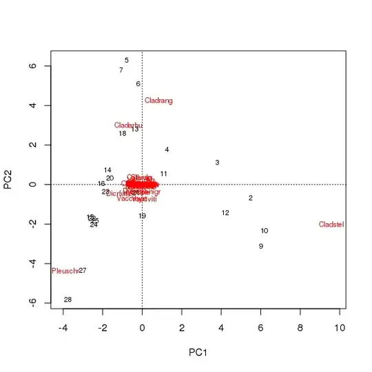
There are two issues here
- The ordination is essentially dominated by three species — these species lie farthest from the origin — as these are the most abundant taxa in the data set
- There is a strong arch of curve in the ordination, suggestive of a long or dominant single gradient that has been broken down into the two main principal components to maintain the metric properties of the ordination.
CA
A CA might assist with both these points as it handles long gradient better due to the unimodal response model, and it models relative composition of species not raw abundances.
The vegan / R code to do this is similar to the PCA code used above
cafit <- cca(varespec)
cafit

> cafit <- cca(varespec)
> cafit
Call: cca(X = varespec)

              Inertia Rank
Total           2.083
Unconstrained   2.083   23
Inertia is mean squared contingency coefficient

Eigenvalues for unconstrained axes:
   CA1    CA2    CA3    CA4    CA5    CA6    CA7    CA8
0.5249 0.3568 0.2344 0.1955 0.1776 0.1216 0.1155 0.0889
(Showed only 8 of all 23 unconstrained eigenvalues)
Here we explain about 40% of the variation among sites in their relative composition
> head(cumsum(eigenvals(cafit)) / cafit$tot.chi)
      CA1       CA2       CA3       CA4       CA5       CA6
0.2519837 0.4232578 0.5357951 0.6296236 0.7148866 0.7732393
The joint plot of the species and site scores is now less dominated by a few species
> plot(cafit)
Which of PCA or CA you choose should be determined by the questions you wish to ask of the data. Usually with species data we are more often interested in difference in the suite of species so CA is a popular choice. If we have a data set of environmental variables, say water or soil chemistry, we wouldn't expect those to respond in a unimodal manner along gradients so CA would be inappropriate and PCA (of a correlation matrix, using scale = TRUE in the rda() call) would be more appropriate.
Constrained ordination; CCA
Now if we have second set of data which we wish to use to explain patterns in the first species data set, we must use a constrained ordination. Often the choice here is CCA, but RDA is an alternative, as is RDA after transformation of the data to allow it to handle species data better.
data(varechem) # load explanatory example data
We re-use the cca() function but we either supply two data frames (X for species, and Y for explanatory/predictor variables) or a model formula listing the form of the model we wish to fit.
To include all variables we could use varechem ~ ., data = varechem as the formula to include all variables — but as I said above, this isn't a good idea in general
ccafit <- cca(varespec ~ ., data = varechem)

> ccafit
Call: cca(formula = varespec ~ N + P + K + Ca + Mg + S + Al + Fe + Mn +
Zn + Mo + Baresoil + Humdepth + pH, data = varechem)

              Inertia Proportion Rank
Total          2.0832     1.0000
Constrained    1.4415     0.6920   14
Unconstrained  0.6417     0.3080    9
Inertia is mean squared contingency coefficient

Eigenvalues for constrained axes:
  CCA1   CCA2   CCA3   CCA4   CCA5   CCA6   CCA7   CCA8   CCA9  CCA10  CCA11
0.4389 0.2918 0.1628 0.1421 0.1180 0.0890 0.0703 0.0584 0.0311 0.0133 0.0084
 CCA12  CCA13  CCA14
0.0065 0.0062 0.0047

Eigenvalues for unconstrained axes:
    CA1     CA2     CA3     CA4     CA5     CA6     CA7     CA8     CA9
0.19776 0.14193 0.10117 0.07079 0.05330 0.03330 0.01887 0.01510 0.00949
The triplot of the above ordination is produced using the plot() method
> plot(ccafit)
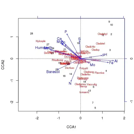
Of course, now the task is to work out which of those variables is actually important. Also note that we have explained about 2/3 of the species variance using just 13 variables. one of the problems of using all variables in this ordination is that we've created an arched configuration in sample and species scores, which is purely an artefact of using too-many correlated variables.
If you want to know more about this, check out the vegan documentation or a good book on multivariate ecological data analysis.
Relationship with regression
It is simplest to illustrate the link with RDA, but CCA is just the same except everything involves row and column two-way-table marginal sums as weights.
At it's heart, RDA is equivalent to the application of PCA to a matrix of fitted values from a multiple linear regression fitted to each species (response) values (abundances, say) with predictors given by the matrix of explanatory variables.
In R we can do this as
## centre the responses
spp <- scale(data.matrix(varespec), center = TRUE, scale = FALSE)
## ...and the predictors
env <- as.data.frame(scale(varechem, center = TRUE, scale = FALSE))

## fit a linear model to each column (species) in spp.
## Suppress intercept as we've centred everything
fit <- lm(spp ~ . - 1, data = env)

## Collect fitted values for each species and do a PCA of that
## matrix
pclmfit <- prcomp(fitted(fit))
The Eigenvalues for these two approaches are equal:
> (eig1 <- unclass(unname(eigenvals(pclmfit)[1:14])))
 [1] 820.1042107 399.2847431 102.5616781  47.6316940  26.8382218  24.0480875
 [7]  19.0643756  10.1669954   4.4287860   2.2720357   1.5353257   0.9255277
[13]   0.7155102   0.3118612
> (eig2 <- unclass(unname(eigenvals(rdafit, constrained = TRUE))))
 [1] 820.1042107 399.2847431 102.5616781  47.6316940  26.8382218  24.0480875
 [7]  19.0643756  10.1669954   4.4287860   2.2720357   1.5353257   0.9255277
[13]   0.7155102   0.3118612
> all.equal(eig1, eig2)
[1] TRUE
For some reason I can't get the axis scores (loadings) to match, but invariably these are scaled (or not) so I need to look into exactly how those are being done here.
We don't do the RDA via rda() as I showed with lm() etc, but we use a QR decomposition for the linear model part and then SVD for the PCA part. But the essential steps are the same.