How do I interpret a variance ratio test in Stata?

Question

I need help with interpreting output from a Variance Ratio Test in Stata.

$f = 1.2988$ (my variance)
$\text{Degrees of freedom} = 249, 493$

I have Ho: ratio = 1 as my null

Ha: ratio != 1 Am I correct in thinking this means that if variances are equal than $f=1$ and therefore there is a significant difference between the two groups?

$2* Pr(F > f) = 0.0155$. As it is less than 0.05 am I correct that I can reject the null?

I'm not sure what this is, since I don't use Stata, but note that using F to test the ratio of 2 variances to determine if the variances are equal is not recommended. See: [Why Levene test of equality of variances rather than F ratio?](http://stats.stackexchange.com/a/24024/7290) Also, you don't have to multiply your p-value by 2 for an F test. — gung - Reinstate Monica, Nov 19 '14 at 15:45
Whenever it's conventional to calculate larger/smaller, the test is one-tailed. Seemingly makes no difference here practically, but the precise context is lacking, yet use of Stata otherwise has no bearing on the answer. @gung's concern is real but orthogonal. — Nick Cox, Nov 19 '14 at 16:16

dimitriy · Answer 1 · 2014-11-21T02:25:01.857

Here's an example using the auto dataset, where we compare the variance of foreign and domestic automobile prices:

. #delimit;
delimiter now ;
. sysuse auto, clear;
(1978 Automobile Data)

. sdtest price, by(foreign);

Variance ratio test
------------------------------------------------------------------------------
   Group |     Obs        Mean    Std. Err.   Std. Dev.   [95% Conf. Interval]
---------+--------------------------------------------------------------------
Domestic |      52    6072.423    429.4911    3097.104    5210.184    6934.662
 Foreign |      22    6384.682    558.9942    2621.915     5222.19    7547.174
---------+--------------------------------------------------------------------
combined |      74    6165.257    342.8719    2949.496    5481.914      6848.6
------------------------------------------------------------------------------
    ratio = sd(Domestic) / sd(Foreign)                            f =   1.3953
Ho: ratio = 1                                    degrees of freedom =   51, 21

    Ha: ratio < 1               Ha: ratio != 1                 Ha: ratio > 1
  Pr(F < f) = 0.7963         2*Pr(F > f) = 0.4073           Pr(F > f) = 0.2037

The observed ratio of variances is $f=1.3953$. Under the null that $R=1$, the variance ratio $R$ is distributed as $F(51,21)$. The degrees of freedom of the $F$ distribution are the numbers of observations in each group less one (since we had to estimate two means). This distribution looks like this:

enter image description here
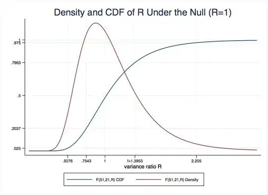
As you can see, the observed ratio is near the center of the distribution, so we are unlikely to reject the null.

More formally, the $p$-value is the probability that we observe a test statistic $R$ at least as large as the one we saw, $f=1.3963$, under the null distribution above. For the one-tailed test where the alternative hypothesis is $R<1$, that is $$P(R < 1.3953)=F(51,21,1.3953)=0.7963.$$ You can read that off from the CDF (blue line) or use the display F(51,21,1.3953) in Stata. For the other two-tailed test, where the alternative is $R>1$, we need $$P(R>1.3953)=1-P(R<1.3953)=0.2037.$$

The two-tailed test is somewhat more complicated. We basically need $P(R>1.3953)=0.2037$, plus the corresponding probability that $R$ is extremely small, which happens to be the same, and corresponds to the probability $P(R<0.7543)=0.2037$. That is why Stata just reports two times the $p$-value for the $H_a:R>1$ one sided test. If we observed that $f<1$, you would use the $p$-value for the other one (try sdtest mpg, by(foreign) for one example).

Finally, @gung and @NickCox's comments about non-robustness of the $F$ test (and Bartlett’s generalization of it to more than two groups) should not be ignored. In Stata, you can implement Levene’s test with:

. robvar price , by(foreign)

            |          Summary of Price
   Car type |        Mean   Std. Dev.       Freq.
------------+------------------------------------
   Domestic |   6,072.423   3,097.104          52
    Foreign |   6,384.682   2,621.915          22
------------+------------------------------------
      Total |   6,165.257   2,949.496          74

W0  =  0.23429053   df(1, 72)     Pr > F = 0.6298296

W50 =  0.00098009   df(1, 72)     Pr > F = 0.97511185

W10 =  0.03306479   df(1, 72)     Pr > F = 0.85622141

The $W_0$ is Levene's robust statistic and $0.6298296$ is the $p$-value for the null that the variances are all equal, with the alternative that at least one pair is not. The $W_{50}$ replaces the group-specific means in the test statistic formula with the medians and $W_{10}$ replaces them with the 10% trimmed mean. There's some simulation evidence that the median performs better in terms of robustness and power when the data are skewed, while the the trimmed mean is well suited for fat-tailed distributions. The mean is intended for symmetric, moderate-tailed distributions. Arguably, the median is the one to use here, though it doesn't matter.

This $W_0$ is distributed $F(1,72)$, so we can calculate the $p$-value as $$1-P(W_0<0.23429053)=.6298296.$$ The degrees of freedom are given by the number of groups less one, and the total number of observations less the number of group-specific means.

How do I interpret a variance ratio test in Stata?

1 Answers1