0

I am not very good in statistics (ok, I'm really bad), I guess this is a very simple question but I dont understand much of the literature.

I have a dataset that is arranged in 2 columns (var1 is my response variable, var2 my predictor). Based on Pearson correlation coefficient, I found that my data is correlated (with a significant p-value < 0.01). I also fitted a regression model in R as lm(var1 ~ var2), and made a nice graph.

If my two variables are correlated, does this mean that I can use the results from my linear regression to make a prediction, or do I have to rely on another technique? What I am trying to predict is the number of failures by time X in the same software. The regression equation I obtained reads $0.002282\cdot x +0.545751$.

The data sample is not very big, it is the cumulative number of failures experienced in a software program through time.

> summary(FAILURES,TOTALTIME)
  Min. 1st Qu.  Median    Mean 3rd Qu.    Max. 
  1.00    4.25    7.50    7.50   10.75   14.00
>cor.test(TOTALTIME,FAILURES)
Pearson's product-moment correlation
data:  TOTALTIME and FAILURES 
t = 54.1572, df = 12, p-value = 8.882e-16
alternative hypothesis: true correlation is not equal to 0 
95 percent confidence interval:
0.9933656 0.9993741 
sample estimates:
cor 
0.9979606 

Here is a graph of my data:

scatterplot with fit

chl
  • 50,972
  • 18
  • 205
  • 364
santiagozky
  • 115
  • 1
  • 4
  • @santiagozky I've made some edits to your question to make it clear that you're trying to predict values from a linear regression model. However, you'll need to clarify some issues: (a) are you trying to predict new (unobserved) values or get the fitted values for your actual observations? (b) can you give more information on model fit (R `summary()` output) or a scatterplot of your data (as a rough check for outliers, etc.)? – chl Jun 27 '11 at 16:50
  • You should mention what kind of data it is and how it was obtained. That would help us answer your question. Statistical methods like lm depend on certain assumptions, and they simply crunch your input through a formula and spit out "answers". If the data does not satisfy lm's assumptions, the answer will be random garbage. So you need to think about the data and the system you are trying to model with a straight line, to see if 55.17 and 19.31 make sense. What would they mean in the real world, and is that plausible? And how did your two columns of data arise? – Wayne Jun 27 '11 at 16:54
  • 1
    The answer is yes and the details are provided at http://stats.stackexchange.com/questions/9131/obtaining-a-formula-for-prediction-limits-in-a-linear-model – whuber Jun 27 '11 at 18:19
  • thanks for suggestions, I added more info and corrected the regression, which was from another case I have. @whuber thanks. I thought this was asked before but I couldnt find it – santiagozky Jun 27 '11 at 19:27
  • 3
    @santiagozky: The description and graph are very helpful because they show this is a time-to-failure problem, not a regression problem. – whuber Jun 27 '11 at 19:37
  • Excellent update! (Unfortunately, your clarification puts the problem into an area that I'm not familiar with.) Two suggestions, though: 1) Look at the time between errors and read up on the Poisson distribution (http://en.wikipedia.org/wiki/Poisson_distribution), and 2) is anything being done to decrease failures or is the software and process for using the software in a steady state? (Most of the software reliability methods I could find assume that bugs are found and fixed, so the curve you've drawn would become less and less steep over time.) – Wayne Jun 27 '11 at 21:03

2 Answers2

1

You have taken count data ( i.e.the number of failures in the first interval , the second interval , the nth interval ) and added them to create a cumulative series which is autocorrelated as a result of your summation strategy. You then try to use a procedure to test the relationship between cumulative failures and cumulative time . Note the procedure you are using requires independent observations while you have autocorrelated observations. A recent reviewerof AUTOBOX, a program I am involved in, made a similar tactical error in trying to correlate/predict a movies total box-office receipts as a function of time. The movie was "Alice in Wonderland" and he should have known better. He constructed the sum of weekly box-office receipts to create a "total box-office-to-date series". Please Google "alice in wonderland box office jack yurkewicz" for details on this. The correct procedure is to analyze the observed time series data and construct an ARIMA Model taking into account any Interventions (Pulses,Level Shifts,Local Time Trends,Seasonal Pulses) that may have occurred

IrishStat
  • 27,906
  • 5
  • 29
  • 55
  • How exactly can this dataset be construed as a time series? – whuber Jun 27 '11 at 20:25
  • @whuber: If you observe 2 failures in the first bucket (first 1000 hours) ; and say 3 failures in the next bucket ( hours between 1000 and 2000) ; etc .. For example 2,3,2,2,2,3,1,0,1,0 for the first ten intervals might suggest a shift in the mean at period 7. – IrishStat Jun 27 '11 at 20:47
  • Thank you. I think it's important to be explicit about the data representation when a problem does not initially appear to be a time series. Your response raises an interesting question that perhaps your experience can help us answer: to what extent would the analysis be sensitive to the choice of bucket sizes? It seems to me, for example, that there would be problems performing an analysis with these particular data using a one-hour bucket. – whuber Jun 27 '11 at 22:08
  • @whuber If you selected a "bucket size" that small then there is a "false autocorrelation" as you will have tons of zeroes and it will appear that one zero can predict another/ When you have "sparse data" or "intermittent demand/failure data" then one has two random variables ( the time bwtween events and the size of the event). Care should be taken to not make the time interval too small or too large. Some judgement is required in not making the interval too fine or too coarse. – IrishStat Jun 27 '11 at 23:16
  • @whuber: On another note I am stunned by the naivety of comments as it relates to interpreting ols/correlation coeeficients when dealing with time series data, as is the case here. It appears to me that some mathematicians often overlook the requirements for testing significance of model parameters when there are Gaussian Violations and they do so at their own peril. – IrishStat Jun 28 '11 at 16:07
1

EDIT AFTER ACCEPTED:

It appears that your rate of failure may be decreasing over time. For example, if you regard this as a time series, it takes two differences to remove the trend, which could indicate a quadratic. And if I do try to fit it as a quadratic (and an lm and a glm):

n <- nls (y ~ a + (b * x) + (c * x^2), start=list (a=0, b=1, c=1))
curve (coef (n)[1] + (coef (n)[2] * x) + (coef (n)[3] * x^2), 0, 6000)
points (x, y)
l <- lm (y ~ x + 0)
g <- glm (y ~ x + 0, family=quasipoisson (link="identity"))
abline (0, coef (g), col="green")
abline (0, coef (l), col="red")

I get:

Quadratic, lm, glm

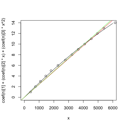
Where the quadratic (black line) looks more reasonable than the other two. (Of course "looks reasonable" does not mean "is correct", and it can't actually be a quadratic because at some point it would begin to decrease which is impossible with a cumulative sum.) In both the lm and glm, your last point is a serious outlier. (I am estimating $x$ from your graph and could be wrong. Including your actual data would be helpful.)

In light of this, it may be that the process is changing as software can: bugs being fixed, people learning to work around bugs, or the environment/process changing so that failures are less likely to be encountered. If this is the case, a linear model wouldn't be appropriate, and these "external forces" would also violate Poisson assumptions, I think.

ORIGINAL: I believe this is basic statistics, but being self-taught I definitely have holes in my statistical knowledge. Never the less, I'll take a stab at it.

First, many models used for software bugs assume that there are a finite number of bugs that are found and each is fixed. Is your case like that? Are bugs being found and fixed in the software, or is the process in which you use the software being modified to work around bugs? If so, the number of failures per 1000 "hours" (I'll call it "hours" since I don't know your X units) will decline over time, and you get into survival time analysis and all kinds of stuff I know nothing about.

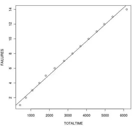
Second, if everything is in a steady state (no bugs being fixed, no process change), your data could be described as a Poisson process. Eyeballing your data, the number of errors per 1000 hours is: 2, 3, 2, 2, 2, 2, which yields an average of 2.17 errors per 1000 hours. (Leaving out the last error beyond 6000.)

Looking at the Wikipedia page for Poisson Distribution, we see that if your error rate is actually Poisson($\lambda$), then $\lambda=2.17$ (the average), and you can plot the odds of getting a given number of errors in 1000 hours as, plot (dpois (0:6, 2.17), type="o"), and the odds of getting a number of errors or fewer in 1000 hours is plot (cumsum (dpois (1:6, 2.17)), type="o").

These odds don't change from 1000-hour period to 1000-hour period, assuming the software and process (and environment, really) are also unchanging and thus a Poisson distribution makes sense.

So, let's extrapolate, and look at your 6000-hour time period. To plot out the distribution for the expected number of errors in that time, plot (dpois (0:30, 2.17 * 6), type="o"), which nicely reflects the 13 errors you actually saw.

Not sure how to carry a Poisson analysis beyond this point.

When I look at the dpois curve, it looks to my eye like it might be close enough to normal; I'm sure there's a test for that and others here could tell us quickly. If it is close enough to normal, it would indicate that the residuals of the lm are normal, which would indicate that lm might be a reasonable thing to do. It doesn't make sense that when $x=0$ you have $y=0.545751$ (i.e. you have half a failure before you even begin). You can prevent this by using lm (var1 ~ var2 + 0), but I'm not sure if that makes sense in this case or not.

Actually, lm, like a Poisson model, assumes that your counts are not related: that the number of failures in any period of time is independent of the number of failures in previous times. You'd want to make sure that's true of your actual failures, otherwise, as IrishStat mentions, you'll get into a time-series situation which is again more complicated.

Wayne
  • 19,981
  • 4
  • 50
  • 99
  • thanks wayne. I will reinterpret my data using a Poisson model. I think that would be a better option. @Irish answer seems good but I'm afraid it surpasses my knowledge by a lot. At least I know a bit about Poisson. – santiagozky Jun 28 '11 at 12:16