This question was explicitly answered in the classical series of papers on James-Stein estimator in the Empirical Bayes context written in the 1970s by Efron & Morris. I am mainly referring to:
Efron and Morris, 1973, Stein's Estimation Rule and Its Competitors -- An Empirical Bayes Approach
Efron and Morris, 1975, Data Analysis with Stein's Estimator and Its Generalizations
Efron and Morris, 1977, Stein's Paradox in Statistics
The 1977 paper is a non-technical exposition that is a must read. There they introduce the baseball batting example (that is discussed in the thread you linked to); in this example the observation variances are indeed supposed to be equal for all variables, and the shrinkage factor $c$ is constant.
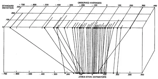
However, they proceed to give another example, which is estimating the rates of toxoplasmosis in a number of cities in El Salvador. In each city different number of people were surveyed, and so individual observations (toxoplasmosis rate in each city) can be thought of having different variances (the lower the number of people surveyed, the higher the variance). The intuition is certainly that data points with low variance (low uncertainty) don't need to be shrunken as strongly as data points with high variance (high uncertainty). The result of their analysis is shown on the following figure, where this can indeed be seen to be happening:
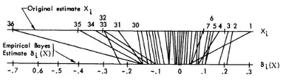
The same data and analysis are presented in the much more technical 1975 paper as well, in a much more elegant figure (unfortunately not showing the individual variances though), see Section 3:
There they present a simplified Empirical Bayes treatment that goes as follows. Let $$X_i|\theta_i \sim \mathcal N(\theta_i, D_i)\\ \theta_i \sim \mathcal N(0, A)$$ where $A$ is unknown. In case all $D_i=1$ are identical, the standard Empirical Bayes treatment is to estimate $1/(1+A)$ as $(k-2)/\sum X_j ^2$, and to compute the a posteriori mean of $\theta_i$ as $$\hat \theta_i = \left(1-\frac{1}{1+A}\right)X_i = \left(1-\frac{k-2}{\sum X_j^2}\right)X_i,$$ which is nothing else than the James-Stein estimator.
If now $D_i \ne 1$, then the Bayes update rule is $$\hat \theta_i = \left(1-\frac{D_i}{D_i+A}\right)X_i$$ and we can use the same Empirical Bayes trick to estimate $A$, even though there is no closed formula for $\hat A$ in this case (see paper). However, they note that
... this rule does not reduce to Stein's when all $D_j$ are equal, and we instead use a minor variant of this estimator derived in [the 1973 paper] which does reduce to Stein's. The variant rule estimates a different value $\hat A_i$ for each city. The difference between the rules is minor in this case, but it might be important if $k$ were smaller.
The relevant section in the 1973 paper is Section 8, and it is a bit of a tougher read. Interestingly, they have an explicit comment there on the suggestion made by @guy in the comments above:
A very simple way to generalize the James-Stein rule for this situation is to define $\tilde x_i = D_i^{-1/2} x_i, \tilde \theta_i = D_i^{-1/2} \theta_i$, so that $\tilde x_i \sim \mathcal N(\tilde \theta_i, 1)$, apply [the original James-Stein rule] to the transformed data, and then transform back to the original coordinates. The resulting rule estimates $\theta_i$ by
$$\hat \theta_i = \left(1-\frac{k-2}{\sum [X_j^2 / D_j]}\right)X_i.$$ This is unappealing since each $X_i$ is shrunk toward the origin by the same factor.
Then they go on and describe their preferred procedure for estimating $\hat A_i$ which I must confess I have not fully read (it is a bit involved). I suggest you look there if you are interested in the details.