This is a bit longish (I want to be thorough), but my actual question is a short one (in bold below).
BACKGROUND: Suppose I have a conditional logistic discrete time event history model (aka logistic discrete time survival models aka logit hazard model) across $p$ possibly time-varying predictors $\mathbf{X} = \{X_{1t}, \dots, X_{pt}\}$ for $T$ time periods indexed by $t$ from $1, \dots, T$ something like:
$$\text{logit}\left(h_{t,\mathbf{X}}\right) = \alpha_{1}d_{1} + \dots + \alpha_{T}d_{t} + \mathbf{BX_{t}},$$
Where $d_{1}, \dots, d_{T}$ are indicator variables of each time period, $\alpha_{1}, \dots, \alpha_{T}$ are the period-specific intercepts for the hazard function, and $\mathbf{BX}$ are the conditionals and their effects. This model implies that the hazard function is
$$h_{t,\mathbf{X}} = \frac{e^{\alpha_{1}d_{1} + \dots + \alpha_{T}d_{T} + \mathbf{BX_{t}}}}{1 + e^{\alpha_{1}d_{1} + \dots + \alpha_{T}d_{T} + \mathbf{BX_{t}}}}= \frac{e^{\alpha_{t}d_{t} + \mathbf{BX_{t}}}}{1 + e^{\alpha_{t}d_{t} + \mathbf{BX_{t}}}}.$$
A success story:
I would like to employ frequentist inference using confidence intervals around my estimated model quantities. So, using the delta method, I can estimate the variance of $\hat{h}_{t,\mathbf{X}}$ as (see end of question for derivation):
$$\sigma^{2}_{\hat{h}_{t}} = \left[\frac{e^{\hat{\alpha}_{t}+\hat{\mathbf{B}}\mathbf{X}_{t}}}{\left(1+e^{\hat{\alpha}_{t}+\hat{\mathbf{B}}\mathbf{X}_{t}}\right)^{2}}\right]^{2}\mathbf{Z}_{t}\mathbf{\Sigma}_{t}\mathbf{Z}_{t}^{\text{T}},$$
Where the $p+1$ row vector $\mathbf{Z}_{t} = \left[d_{t},\mathbf{X}_{t}\right]$, and $\mathbf{\Sigma}_{t}$ is the variance-covariance matrix of $\mathbf{Z}_{t}$.
When I run simulations of Wald-type confidence intervals ($\hat{h}_{t,\mathbf{X}} \pm t_{\text{CI}}\sigma^{2}_{\hat{h}_{t,\mathbf{X}}}$) using this variance estimator for unconditional models, for models conditioned on two variables, and for models conditioned on those variables plus an interaction (aside: also using different parameterizations of time, more about those at the very end), I get coverage probabilities very close to the nominal confidence level at each time period (i.e. CI of 0.9, 0.95, and 0.99). For example, here are the coverage probabilities across 9 models with a nominal 95% confidence level:

Woot! That looks swell.
A failure story:
The survivor function, $S_{t,\mathbf{X}}$ is also an important quantity in event history models:
$$\hat{S}_{t,\mathbf{X}} = \prod_{i=1}^{t}{\left(1-\hat{h}_i\right)} = \prod_{i=1}^{t}{\frac{1}{1+e^{\hat{\alpha}_{i}+\hat{\mathbf{B}}\mathbf{X}_{i}}}}$$
However, when I go on to derive the variance of the survival function using the delta method to get (see end of question for derivation):
$$\sigma^{2}_{\hat{S}_{t}} = \left[\sum_{i=1}^{t} { \mathbf{Z}_{i}{\mathbf{\Sigma}_{i}}\mathbf{Z}_{i}^{\mathrm{T}} \left(\frac{e^{\hat{\alpha}_{i}+\hat{\mathbf{B}}\mathbf{X}_{i}}}{1+e^{\hat{\alpha}_{i}+\hat{\mathbf{B}}\mathbf{X}_{i}}}\right)^{2}}\right] \left[\prod_{i=1}^{t}{\left(\frac{1}{1+e^{\hat{\alpha}_{i}+\hat{\mathbf{B}}\mathbf{X}_{i}}}\right)}\right]^{2}$$
My coverage probabilities are badly biased. For example, here are the coverage probabilities across 9 models with a nominal 95% confidence level (YUCK!):
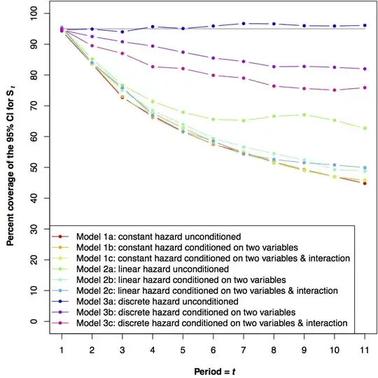
I have played around with multiple comparisons adjustments at each succeeding time period... but something fundamental is eluding me. I and a colleague have checked the simulations together, and implemented them in R and Stata so we don't think it is a programming error.
QUESTION: Why am I not getting proper coverage probabilities on $\hat{S}_{t}$ for any but unconditional models with fully discrete parameterizations of time?
Brainstorms are welcome. "You forgot to carry the 2"-type ideas are welcome. Hints are welcome. "Assumption of independence is inappropriate because..." is welcome.
Derivation of $\sigma^{2}_{\hat{h}_{t}}$ using a first-order delta-method approximation:
$$\mathbf{V}_{t} = \left.\left[\begin{array}{cccc}\frac{{\partial}h_{t}}{{\partial}\alpha_{t}} & \frac{{\partial}h_{t}}{{\partial}\beta_{1}} & \cdots & \frac{{\partial}h_{t}}{{\partial}\beta_{p}}\end{array}\right]\right|_{\alpha_{t} = \hat{\alpha}_{t}, \mathbf{B} = \hat{\mathbf{B}}}\\
\\
= \left[\begin{array}{ccc}\frac{e^{\left(\hat{\alpha}_{t}+\hat{\mathbf{B}}\mathbf{X}_{t}\right)}}{\left(1+e^{\left(\hat{\alpha}_{t}+\hat{\mathbf{B}}\mathbf{X}_{t}\right)}\right)^{2}} & \frac{X_{1t}e^{\left(\hat{\alpha}_{t}+\hat{\mathbf{B}}\mathbf{X}_{t}\right)}}{\left(1+e^{\left(\hat{\alpha}_{t}+\hat{\mathbf{B}}\mathbf{X}_{t}\right)}\right)^{2}} & \cdots & \frac{X_{pt}e^{\left(\hat{\alpha}_{t}+\hat{\mathbf{B}}\mathbf{X}_{t}\right)}}{\left(1+e^{\left(\hat{\alpha}_{t}+\hat{\mathbf{B}}\mathbf{X}_{t}\right)}\right)^{2}}\end{array}\right]\\
\\
= \frac{e^{\left(\hat{\alpha}_{t}+\hat{\mathbf{B}}\mathbf{X}_{t}\right)}}{\left(1+e^{\left(\hat{\alpha}_{t}+\hat{\mathbf{B}}\mathbf{X}_{t}\right)}\right)^{2}}\left[\begin{array}{cccc}1 & X_{1t} & \cdots & X_{pt}\end{array}\right]$$
$$\sigma^{2}_{\hat{h}_{t,\mathbf{X}}} = \mathbf{V}_{t}\mathbf{\Sigma}_{t}\mathbf{V}_{t}^{\mathrm{T}} \nonumber\\ = \left[\frac{e^{\left(\hat{\alpha}_{t}+\hat{\mathbf{B}}\mathbf{X}_{t}\right)}}{\left(1+e^{\left(\hat{\alpha}_{t}+\hat{\mathbf{B}}\mathbf{X}_{t}\right)}\right)^{2}}\right]^{2}\left[\begin{array}{cccc}1 & X_{1t} & \cdots & X_{pt}\end{array}\right]\mathbf{\Sigma}_{t}\left[\begin{array}{c}1 \\ X_{1t} \\ \vdots \\ X_{pt}\end{array}\right] \\ \\ = \left[\frac{e^{\hat{\alpha}_{t}+\hat{\mathbf{B}}\mathbf{X}_{t}}}{\left(1+e^{\hat{\alpha}_{t}+\hat{\mathbf{B}}\mathbf{X}_{t}}\right)^{2}}\right]^{2}\mathbf{Z}_{t}\mathbf{\Sigma}_{t}\mathbf{Z}_{t}^{\text{T}}$$
Derivation of $\sigma^{2}_{\hat{S}_{t},\mathbf{X}}$ using a first-order delta method approximation:
We start by making $S_{t,\mathbf{X}}$ more tractable by taking the log and assuming (since $h_{t,\mathbf{X}}$ is conditioned on survival to $t$):
$$\sigma^{2}_{\ln(\hat{S}_{t,\mathbf{X}})} = \sigma^{2}_{\sum_{i=1}^{t}{\ln\left(1-\hat{h}_{i,\mathbf{X}}\right)}}\\
\\
= \sum_{i=1}^{t}{\sigma^{2}_{\ln\left(1-\hat{h}_{i,\mathbf{X}}\right)}} \quad \mathrm{(by\phantom{0}independence)}$$
Then we get down: $$\sigma^{2}_{\hat{S}_{t,\mathbf{X}}} = \left[\sum_{i=1}^{t}{\sigma^{2}_{\hat{h}_{i,\mathbf{X}}}\left(\frac{1}{\hat{h}_{i,\mathbf{X}}-1}\right)^{2}}\right]\hat{S}_{t,\mathbf{X}}^{2} \\ \\ = \left[\sum_{i=1}^{t}{\mathbf{V}_{i}{\mathbf{\Sigma}_{i}}\mathbf{V}_{i}^{\mathrm{T}}\left(\frac{1}{\hat{h}_{i,\mathbf{X}}-1}\right)^{2}}\right]\hat{S}_{t,\mathbf{X}}^{2}\\ \\ = \left[\sum_{i=1}^{t}{\mathbf{V}_{i}{\mathbf{\Sigma}_{i}}\mathbf{V}_{i}^{\mathrm{T}}\left(1+e^{\hat{\alpha}_{i}+\hat{\mathbf{B}}\mathbf{X}_{i}}\right)^{2}}\right]\hat{S}_{t,\mathbf{X}}^{2}\\ \\ = \left[\sum_{i=1}^{t}{\left[\begin{array}{cccc} 1 & X_{1i} & \cdots & X_{pi}\end{array}\right]\mathbf{\Sigma}_{i}\left[\begin{array}{c}1 \\ X_{1i} \\ \vdots \\ X_{pi}\end{array}\right]\left(\frac{e^{\hat{\alpha}_{i}+\hat{\mathbf{B}}\mathbf{X}_{i}}}{1+e^{\hat{\alpha}_{i}+\hat{\mathbf{B}}\mathbf{X}_{i}}}\right)^{2}}\right] \times \left[\prod_{i=1}^{t}{\left(\frac{1}{1+e^{\hat{\alpha}_{i}+\hat{\mathbf{B}}\mathbf{X}_{i}}}\right)}\right]^{2}\\ \\ \sigma^{2}_{\hat{S}_{t,\mathbf{X}}} = \left[\sum_{i=1}^{t} { \mathbf{Z}_{i}{\mathbf{\Sigma}_{i}}\mathbf{Z}_{i}^{\mathrm{T}} \left(\frac{e^{\hat{\alpha}_{i}+\hat{\mathbf{B}}\mathbf{X}_{i}}}{1+e^{\hat{\alpha}_{i}+\hat{\mathbf{B}}\mathbf{X}_{i}}}\right)^{2}}\right] \left[\prod_{i=1}^{t}{\left(\frac{1}{1+e^{\hat{\alpha}_{i}+\hat{\mathbf{B}}\mathbf{X}_{i}}}\right)}\right]^{2}$$
Alternate parameterizations of time:
The derivations and definitions above are given in terms of a fully discrete paramaterization of time (i.e. the $\alpha_{t}d_{t}$ terms).
In the case of a constant effect of time, the $\alpha_{t}d_{t}$ terms are replaced with a single $\beta_{0}$ term.
In the case of a linear effect of time the $\alpha_{t}d_{t}$ terms are replaced with the terms $\beta_{0} + \beta_{1}t$.
$\mathbf{Z}_{t}$ and $\mathbf{\Sigma}_{t}$ are redefined as appropriate in these cases.